Graphical User Interface

This chapter introduces the functionality and usage considerations of the BDF graphical interface.

Initial Parameters Interface

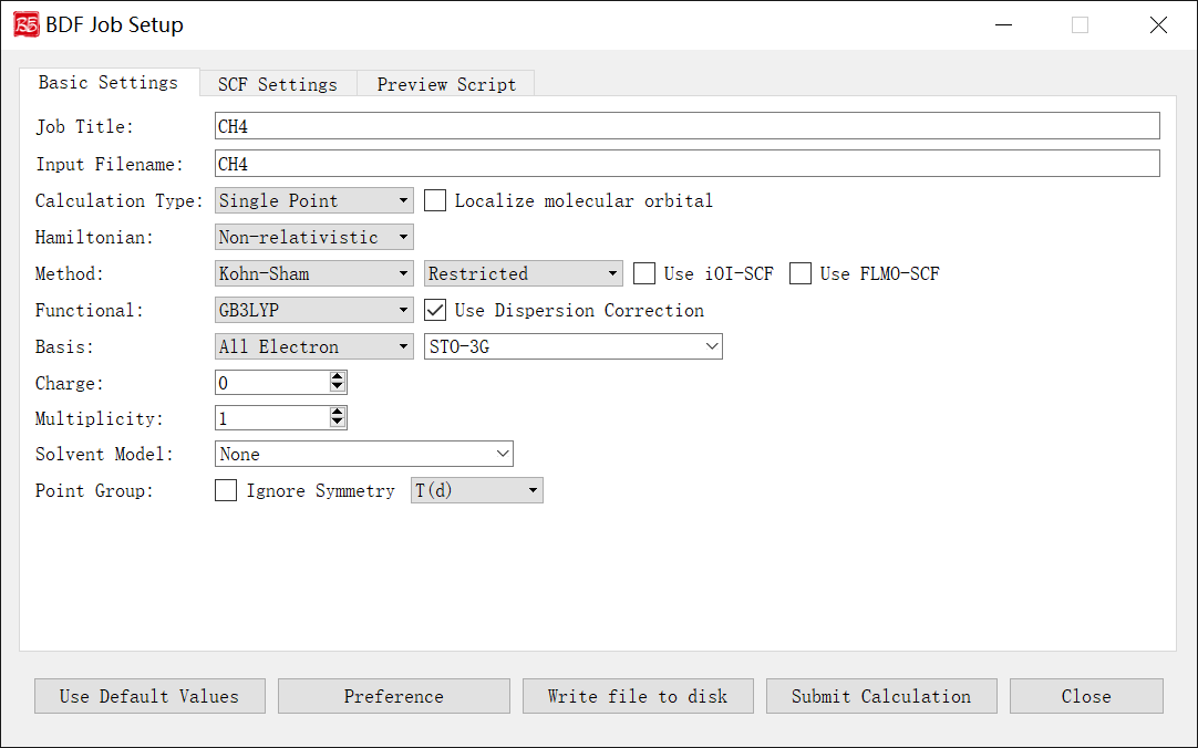
The figure above shows the initial parameters interface when launching the BDF task submission interface, using methane molecule \(\ce{CH4}\) as an example.

After importing the molecular structure, the program automatically identifies chemical formula, charge, symmetry point group, etc., and sets default values for Job Title, Input Filename, Multiplicity, Point Group dropdown, etc.

Controls and functions: 1. Job Title: Task description (e.g., calculation type/molecule/parameters). Does not affect computation but recommended for documentation. Example: SP_CH4_B3LYP-D3/6-31g**. 2. Input Filename: Filename for the task (allowed: letters/numbers/underscores/plus/minus). Example: CH4 → saves as CH4.inp. 3. Calculation Type: Supported types: Single Point, Optimization, Frequency, Opt+Freq, TDDFT, TDDFT-SOC, TDDFT-NAC, TDDFT-OPT, TDDFT-Freq, TDDFT-OPT+Freq, NMR. The Localize molecular orbital checkbox enables orbital localization parameters. Each type activates relevant control modules. 4. Hamiltonian: Relativistic treatment options: Non-relativistic, ECP, sf-X2C. X2C is currently disabled pending future release updates. 5. Method:

• First dropdown: Hartree-Fock, Kohn-Sham, MP2 (MP2 only for single-point).

• Second dropdown: Restricted (closed-shell), Unrestricted (open-shell), Restricted Open (RO).

• Use iOI-SCF/Use FLMO-SCF: Enable fragmentation-based SCF for large systems (single-point only). For geometry optimization, first run iOI/FLMO-SCF then read orbitals as guess.

6. Functional: DFT functional selection (visible only for Kohn-Sham). Lists only functionals compatible with the selected task type. Use Dispersion Correction enables D3 correction if supported.

7. Basis: Basis set type (all-electron, ECP, or custom mix). Restricted to relativistic-optimized basis sets for sf-X2C calculations.

8. Charge: Total molecular charge.

9. Multiplicity: Spin multiplicity (2S+1).

10. Solvent Model: Solvation model.

11. Point Group: Molecular symmetry point group.

SCF Calculation Parameters Interface

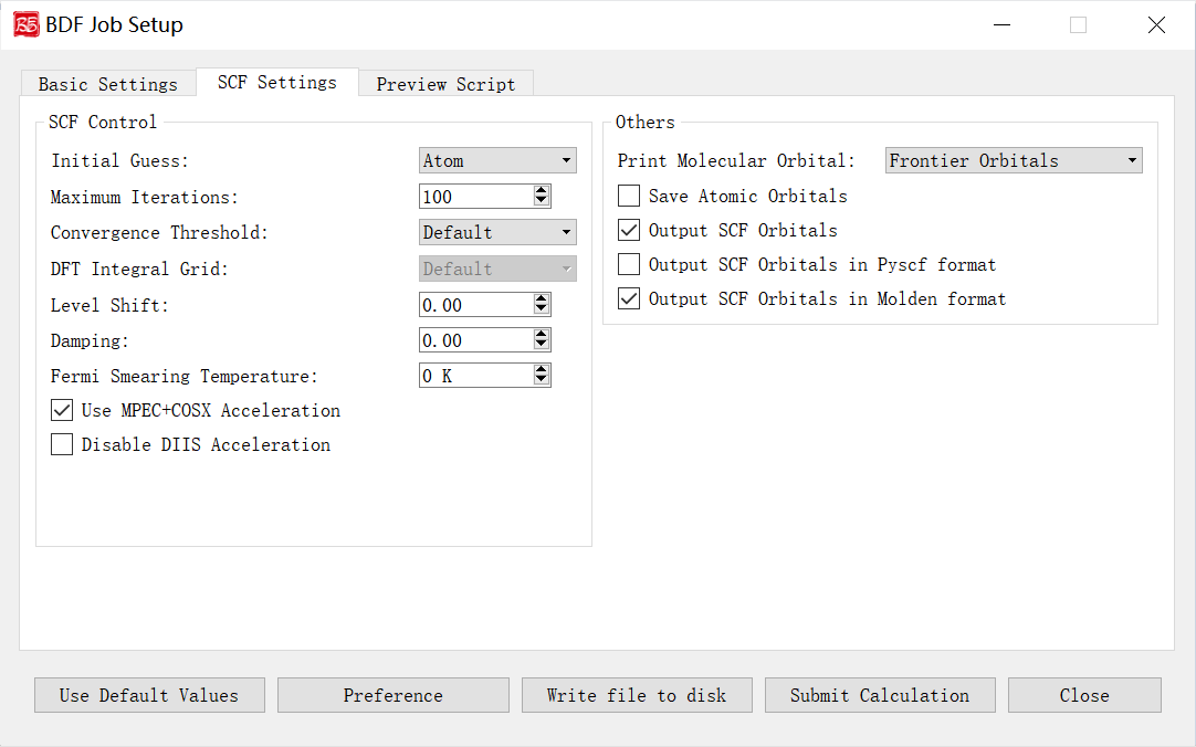
Controls and functions: 1. Initial Guess: Options: Atom (atomic density matrix), Huckel (semi-empirical), Hcore (core Hamiltonian diagonalization), Read (read orbitals). Atom is generally preferred. 2. Maximum Iterations: Max SCF iterations. 3. Convergence Threshold: Energy/density matrix thresholds. Options: Very Tight (1E-10/5E-8), Tight (1E-9/5E-7), Default (1E-7/5E-5), Loose (1E-7/5E-5), Very Loose (1E-6/5E-4). 4. DFT Integral Grid: Grid type for DFT integrals. Options: Default, Ultra Coarse, Coarse, Medium, Fine, Ultra Fine (visible only for Kohn-Sham). 5. Level Shift: Energy shift for virtual orbitals (Vshift). Increases HOMO-LUMO gap to damp oscillations. Use when gap <2 eV or SCF oscillates. 6. Damping: Density mixing (Damp = C). Slows convergence but stabilizes oscillations. Formula: P(i) = (1-C)*P(i) + C*P(i-1). 7. Fermi Smearing Temperature: Electronic temperature for fractional occupation. Disabled if Vshift >0 or for FLMO/iOI calculations. 8. Use MPEC+COSX Acceleration: Accelerates J/K matrices via multipole expansion (MPEC) and chain-of-spheres exchange (COSX). Recommended for >20 atoms. 9. Disable DIIS Acceleration: Disables DIIS convergence accelerator. Use if SCF oscillates severely (>1E-5) and damping/shift fail. 10. Print Molecular Orbital: Options: Frontier Orbitals (HOMO-5 to LUMO+5), Energy & Occupation, All Information. 11. Save Atomic Orbitals: Compute/store atomic orbitals. 12. Output SCF Orbitals: Write converged orbitals to .scforb file (uncheck to disable). 13. Output SCF Orbitals in Pyscf format: Save orbitals in Pyscf format. 14. Output SCF Orbitals in Molden format: Export orbitals in Molden format for analysis.

Geometry Optimization Parameters Interface

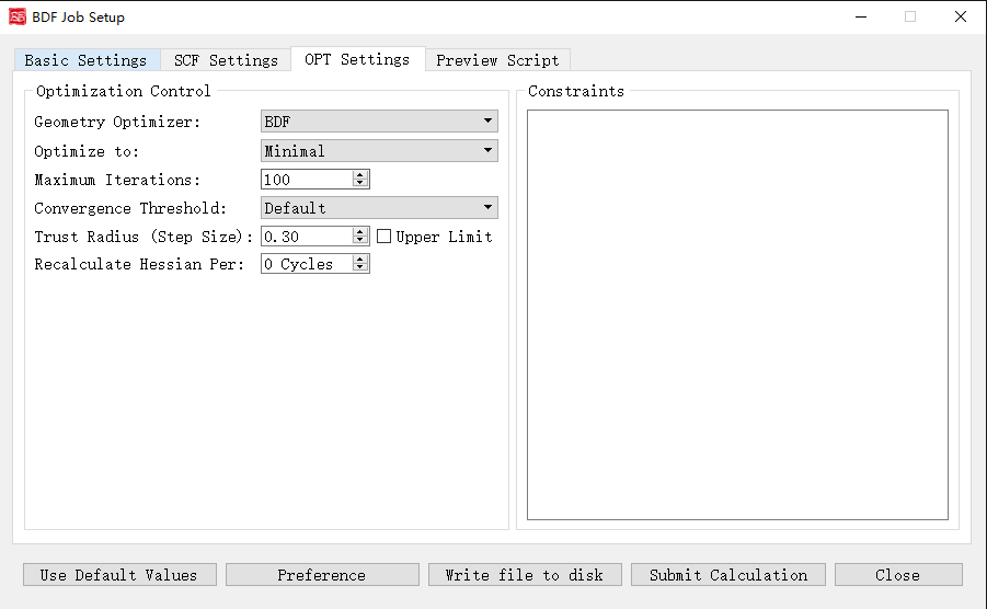
Activated for: Optimization, Opt+Freq, TDDFT-OPT, TDDFT-OPT+Freq.

Controls and functions: 1. Geometry Optimizer: DL-Find (supports Cartesian/internal coordinates, TS search, MECP) or BDF (recommended for redundant internal coordinates). 2. Optimize to: Minimal (minima) or Transition State (TS). 3. Maximum Iterations: Max optimization steps. 4. Convergence Threshold: RMS gradient/displacement thresholds. Options: Very Tight, Tight, Default, Loose, Very Loose. 5. Trust Radius (Step Size): Initial trust radius (updated dynamically). Upper Limit caps the radius at |r|. 6. Recalculate Hessian Per: Frequency of numerical Hessian recalculation. 7. Constraints: Freeze bonds/angles/dihedrals (BDF optimizer only). Format: First line = number of constraints N, followed by N lines of 2-4 atom indices (bond/angle/dihedral).

Frequency Calculation Parameters Interface

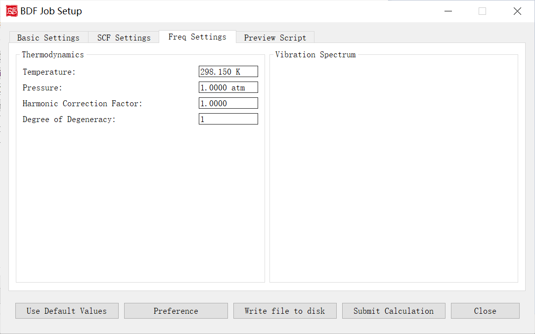
Activated for: Frequency, Opt+Freq, TDDFT-Freq, TDDFT-OPT+Freq.

Controls and functions: 1. Temperature: Temperature for thermochemical analysis. 2. Pressure: Pressure for thermochemical analysis. 3. Harmonic Correction Factor: Frequency scaling factor. 4. Degree of Degeneracy: Electronic degeneracy (g_e) for Gibbs free energy. g_e = spatial degeneracy × spin degeneracy. For Abelian groups, spatial degeneracy=1; spin degeneracy = 2S+1 (non-relativistic/scalar relativistic) or 2J+1 (with SOC). Must be manually set for open-shell systems.

TDDFT Calculation Parameters Interface

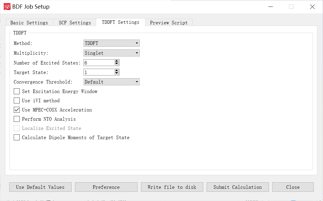
Activated for: TDDFT, TDDFT-SOC, TDDFT-NAC, TDDFT-OPT, TDDFT-Freq, TDDFT-OPT+Freq.

Controls and functions: 1. Method: TDDFT or TDA. 2. Multiplicity: Excited state multiplicity. Options depend on ground state multiplicity:

• Singlet ground: Singlet, Triplet, Singlet & Triplet

• Doublet ground: Doublet, Quartet, Doublet & Quartet

3. Delta Ms: Spin-flip control. `0`=spin-conserving, `1`=spin-up flip, `-1`=spin-down flip. Enabled for multiplicity >2.

4. Number of Excited States: Number of states to compute.

5. Target State: State index for dipole moment calculation (requires Calculate Dipole Moments of Target State).

6. Convergence Threshold: Energy/wavefunction thresholds. Options: Very Tight (1E-9/1E-7), Tight (1E-8/1E-6), Default (1E-7/1E-5), Loose (1E-6/1E-4), Very Loose (1E-5/1E-3).

7. Set Excitation Energy Window: Compute states within specified energy/wavelength range.

8. Use iVI method: Iterative eigensolver for high-energy states or energy-window calculations (not for non-Abelian groups).

9. Use MPEC+COSX Acceleration: Accelerates J/K matrices (recommended for >20 atoms).

10. Perform NTO Analysis: Natural Transition Orbital analysis (Abelian groups only).

11. Localize Excited State: Localized excited states (disabled in GUI; edit input file manually).

12. Calculate Dipole Moments of Target State: Compute transition dipole moments for the target state.

Molecular Orbital Localization Interface

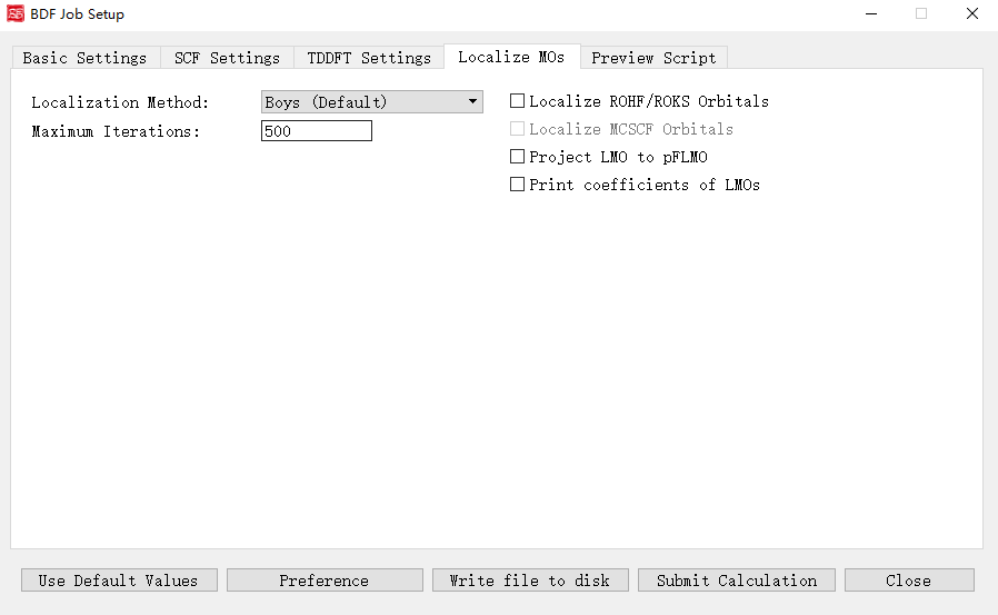
Activated when Localize molecular orbital is checked.

Controls and functions: 1. Localization Method: Boys (Default), Modified Boys, Four-center moment, Pipek-Mezey. 2. Exponential Factor: Exponent for Modified Boys/Four-center moment. 3. Atomic Charge: Mulliken or Lowdin (for Pipek-Mezey). 4. Pipek-Mezey Method: Jacobi Sweep or Trust Region. 5. Maximum Iterations: Max localization cycles. 6. Localize ROHF/ROKS Orbitals: Localize ROHF/ROKS orbitals. 7. Localize MCSCF Orbitals: Localize MCSCF orbitals (disabled pending future release). 8. Project LMO to pFLMO: Project localized MOs to pFLMOs. 9. Print coefficients of LMOs: Print localized orbital coefficients.

Spin-Orbit Coupling Parameters Interface

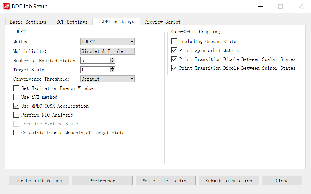
Activated for TDDFT-SOC tasks.

Controls and functions: 1. Including Ground State: Include ground state in SOC calculation. Enables SOC-corrected spectra and ground-state SOC correction (limit: 10-100 states). Disabling excludes ground-spinor transitions. 2. Print Spin-orbit Matrix: Compute and print SOC matrix elements. 3. Print Transition Dipole Between Scalar States: Print all scalar-state transition dipoles. 4. Print Transition Dipole Between Spinor States: Print spinor-state transition dipoles (with oscillator strengths/radiative rates).

Non-Adiabatic Coupling Parameters Interface

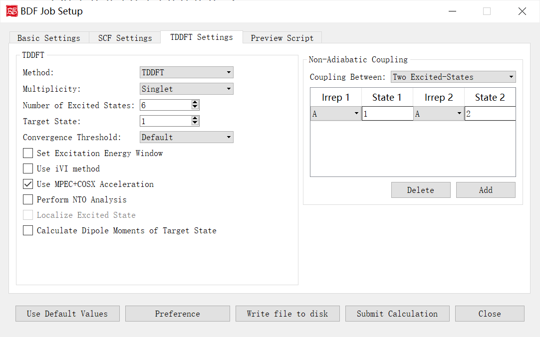
The above figure shows the non-adiabatic coupling calculation parameter interface that starts the BDF task submission interface, that is, the Non-Adiabatic Coupling part of the parameters, and the previous calculation task selects TDDFT-NAC (non-adiabatic coupling calculation), the interface module will be activated.

Let’s explain the controls and functions of the GUI in the above figure:

1. Coupling Between: Specifies which non-adiabatic coupling matrix elements between electronic states are calculated (including non-adiabatic coupling matrix elements between ground state-excited states, and non-adiabatic coupling matrix elements between excited state-excited states). The drop-down box supports Ground and Excited-State and Two Excited-States. Irrep 1 and State 1 specify the irreducible representations of the excited state and the roots of the irreducible representations, respectively, and are used to specify the calculation of the ground-excited state adiabatic coupling vectors. Irrep, State 1, and Irrep and State 2 specify the irreducible representations of the two sets of excited states and the roots of the irreducible representations, respectively, which are used to specify the calculation of the excited state-excited state non-adiabatic coupling vectors.