Get started quickly

This chapter introduces the basic use of BDF’s various functions, and provides basic examples and data reading and analysis instructions for specific calculation functions.

Note

BDF english manual is transfered from chinese manual by AI tool. It is still in checking and improving.

First Example: RHF Calculation of $\ce{H2O}$ Molecule

Hartree-Fock is the most fundamental algorithm in quantum chemistry. In this section, we will guide users performing a Hartree-Fock calculation of a water molecule using BDF. The input and output of BDF will be analysised. We first present the easy input for BDF. To help users understand the difference between BDF’s easy and advanced input modes, we also provide the corresponding advanced input file for each easy input. Notice that the easy input of BDF is still in developing. At present, the adavanced input mode is usually used.

Preparing Input

First, prepare the input file for the single-point energy Hartree-Fock calculation of a water molecule, named h2o.inp. The input content is as follows:

#!bdf.sh
HF/3-21G

Geometry
O
H  1  R1
H  1  R1  2 109.

R1=1.0     # input bond length with the default unit angstrom
End geometry

Interpretation of the input: - The first line must start with #!, followed by a string named bdf.sh. This can be any alphanumeric string and may contain . but no other special characters. This is a system-reserved line; users can use this string to tag the calculation job. - The second line HF/3-21G is BDF’s calculation parameter control line. HF is the abbreviation for Hartree-Fock, and 3-21G specifies the basis set. Key parameter control lines can span multiple consecutive lines. - The third line is blank and can be ignored. It is used here to separate different input sections for readability and is recommended. - Lines 4 and 10 are Geometry and End geometry, marking the start and end of molecular geometry input. The default unit for coordinates is Angstrom. - Lines 5 to 9 input the water molecule structure in Z-matrix (internal coordinate) format (details in Molecular Structure Input in Internal Coordinates).

The corresponding advanced input for this simple input is:

$compass
Geometry
  O
  H 1 1.0
  H 1 1.0 2 109.
End geometry
Basis
  3-21g  # set basis set as 3-21g
$end

$xuanyuan
$end

$scf
RHF       # Restricted Hartree-Fock method
Charge    # Molecular charge set to 0 (default for neutral molecules)
  0
Spinmulti # Spin multiplicity 2S+1 (defaults to singlet for even-electron systems)
  1
$end

From the advanced input, it can be seen that BDF will sequentially execute the COMPASS, XUANYUAN, and SCF modules to complete the single-point energy calculation of the water molecule. COMPASS reads molecular structure, basis functions, and other basic information, determines molecular symmetry, rotates the molecule to standard orientation (see BDF’s Use of Group Theory), generates symmetry-adapted orbitals, etc., and stores this information in the file h2o.chkfil in the execution directory. Key elements in COMPASS: * Molecular structure defined between Geometry and End geometry; * Basis set defined as 3-21G via Basis.

Note

Only in the easy input can variables (e.g., R1 in the example) be used to define internal coordinates and assign values later. Advanced input requires direct numerical definition of internal coordinates; variables are not supported.

After executing COMPASS, BDF uses XUANYUAN to compute one- and two-electron integrals. On default, BDF performs Integral Direct SCF calculation, where the two-electron respulsion integrals (2e-ERIs) are recomputed as needed in each SCF iteration. Therefore, only one-electron integrals are calculated in xuanyuan and 2e-ERIs will be skipped.

Finally, BDF executes the SCF module to perform the self-consistent field (SCF) calculation based on Hartree-Fock: * RHF specifies the Restricted Hartree-Fock method; * Charge sets the system charge to 0; * Spinmulti sets the spin multiplicity to 1.

Here, RHF is mandatory. Charge and Spinmulti can be omitted for restricted methods.

Executing the Calculation

To run the calculation, prepare a shell script named run.sh in the same directory as the input file h2o.inp. The content is:

#!/bin/bash

# Set BDF installation directory
export BDFHOME=/home/bsuo/bdf-pkg-pro
# Set temporary file directory
export BDF_TMPDIR=/tmp/$RANDOM

# Set unlimited stack memory (may be restricted by system on HPC)
ulimit -s unlimited
# Set unlimited CPU time (may be restricted by system on HPC)
ulimit -t unlimited

# Set OpenMP threads
export OMP_NUM_THREADS=4
# Set OpenMP stack size
export OMP_STACKSIZE=1024M

# Execute BDF (output defaults to stdout)
$BDFHOME/sbin/bdfdrv.py -r h2o.inp

This Bash Shell script defines environment variables and uses $BDFHOME/sbin/bdfdrv.py to run the calculation. Key environment variables: * BDFHOME: BDF installation directory; * BDF_TMPDIR: Temporary file directory; * ulimit -s unlimited: Unlimited stack memory; * ulimit -t unlimited: Unlimited execution time; * export OMP_NUM_THREADS=4: Use 4 OpenMP threads; * export OMP_STACKSIZE=1024M: Set stack memory to 1024 MB per thread.

Execute the calculation with:

$ ./run.sh h2o.inp &>h2o.out&

Since BDF prints output to stdout, we redirect it to h2o.out.

Analyzing Results

After calculation, files h2o.out, h2o.chkfil, and h2o.scforb are generated: * h2o.out: Text file containing human-readable output; * h2o.chkfil: Binary file for data transfer between BDF modules; * h2o.scforb: Text file storing SCF molecular orbital coefficients, orbital energies, etc., used for restarts or as initial guesses.

If the easy input is used, h2o.out first displays basic settings:

|================== BDF Control parameters ==================|

  1: Input BDF Keywords
    soc=None    scf=rhf    skeleton=True    xcfuntype=None
    xcfun=None    direct=True    charge=0    hamilton=None
    spinmulti=1

  2: Basis sets
     ['3-21g']

  3: Wavefunction, Charges and spin multiplicity
    charge=0    nuclearcharge=10    spinmulti=1

  5: Energy method
     scf

  7: Acceleration method
     ERI

  8: Potential energy surface method
     energy

|============================================================|

Here: * Input BDF Keywords lists key control parameters; * Basis set shows the basis set; * Wavefunction, Charges and spinmulti shows charge, total nuclear charge, and spin multiplicity (2S+1); * Energy method specifies the energy calculation method; * Acceleration method shows the two-electron integral acceleration method; * Potential energy surface method indicates a single-point calculation.

Next, the COMPASS module starts:

|************************************************************|

    Start running module compass
    Current time   2021-11-18  11:26:28

|************************************************************|

It prints Cartesian coordinates (in Bohr) and basis function details:

|---------------------------------------------------------------------------------|

 Atom   Cartcoord(Bohr)               Charge Basis Auxbas Uatom Nstab Alink  Mass
  O     0.000000  0.000000  0.000000  8.00    1     0     0     0   E     15.9949
  H     1.889726  0.000000  0.000000  1.00    2     0     0     0   E      1.0073
  H    -0.615235  1.786771  0.000000  1.00    2     0     0     0   E      1.0073

|----------------------------------------------------------------------------------|

  End of reading atomic basis sets ..
 Printing basis sets for checking ....

 Atomic label:  O   8
 Maximum L  1 6s3p ----> 3s2p NBF =   9
 #--->s function
      Exp Coef          Norm Coef       Con Coef
           322.037000   0.192063E+03    0.059239    0.000000    0.000000
            48.430800   0.463827E+02    0.351500    0.000000    0.000000
            10.420600   0.146533E+02    0.707658    0.000000    0.000000
             7.402940   0.113388E+02    0.000000   -0.404454    0.000000
             1.576200   0.355405E+01    0.000000    1.221562    0.000000
             0.373684   0.120752E+01    0.000000    0.000000    1.000000
 #--->p function
      Exp Coef          Norm Coef       Con Coef
             7.402940   0.356238E+02    0.244586    0.000000
             1.576200   0.515227E+01    0.853955    0.000000
             0.373684   0.852344E+00    0.000000    1.000000


 Atomic label:  H   1
 Maximum L  0 3s ----> 2s NBF =   2
 #--->s function
      Exp Coef          Norm Coef       Con Coef
             5.447178   0.900832E+01    0.156285    0.000000
             0.824547   0.218613E+01    0.904691    0.000000
             0.183192   0.707447E+00    0.000000    1.000000

Molecular symmetry is automatically determined, and coordinates are rotated to standard orientation:

Auto decide molecular point group! Rotate coordinates into standard orientation!
Threshold= 0.10000E-08 0.10000E-11 0.10000E-03
geomsort being called!
gsym: C02V, noper=    4
Exiting zgeomsort....
Representation generated
Binary group is observed ...
Point group name C(2V)                       4
User set point group as C(2V)
 Largest Abelian Subgroup C(2V)                       4
 Representation generated
 C|2|V|                    2

Symmetry check OK
Molecule has been symmetrized
Number of symmery unique centers:                     2
|---------------------------------------------------------------------------------|

 Atom   Cartcoord(Bohr)               Charge Basis Auxbas Uatom Nstab Alink  Mass
  O     0.000000  0.000000  0.000000  8.00    1     0     0     0   E     15.9949
  H     1.889726  0.000000  0.000000  1.00    2     0     0     0   E      1.0073
  H    -0.615235  1.786771  0.000000  1.00    2     0     0     0   E      1.0073

|----------------------------------------------------------------------------------|

 Atom   Cartcoord(Bohr)               Charge Basis Auxbas Uatom Nstab Alink  Mass
  O     0.000000 -0.000000  0.219474  8.00    1     0     0     0   E     15.9949
  H    -1.538455  0.000000 -0.877896  1.00    2     0     0     0   E      1.0073
  H     1.538455 -0.000000 -0.877896  1.00    2     0     0     0   E      1.0073

|----------------------------------------------------------------------------------|

Note: The final coordinates differ from the input due to symmetry rotation. COMPASS then generates symmetry-adapted orbitals, prints dipole/quadrupole irreps, multiplication table, and orbital counts:

Number of irreps:    4
IRREP:   3   4   1
DIMEN:   1   1   1

 Irreps of multipole moment operators ...
 Operator  Component    Irrep       Row
  Dipole       x           B1          1
  Dipole       y           B2          1
  Dipole       z           A1          1
  Quadpole     xx          A1          1
  Quadpole     xy          A2          1
  Quadpole     yy          A1          1
  Quadpole     xz          B1          1
  Quadpole     yz          B2          1
  Quadpole     zz          A1          1

 Generate symmetry adapted orbital ...
 Print Multab
  1  2  3  4
  2  1  4  3
  3  4  1  2
  4  3  2  1

|--------------------------------------------------|
          Symmetry adapted orbital

  Total number of basis functions:      13      13

  Number of irreps:   4
  Irrep :   A1        A2        B1        B2
  Norb  :      7         0         4         2
|--------------------------------------------------|

Here, the C₂ᵥ point group has 4 irreps (A1, A2, B1, B2) with 7, 0, 4, 2 symmetry-adapted orbitals.

Attention

Different quantum chemistry software may use different standard orientations, potentially labeling molecular orbitals with different irreps.

COMPASS concludes:

|******************************************************************************|

    Total cpu     time:          0.00  S
    Total system  time:          0.00  S
    Total wall    time:          0.02  S

    Current time   2021-11-18  11:26:28
    End running module compass
|******************************************************************************|

Note

Each BDF module prints start/end times for easy error diagnosis.

Next, the XUANYUAN module computes one-electron integrals. Key output:

[aoint_1e]
  Calculating one electron integrals ...
  S T and V integrals ....
  Dipole and Quadupole integrals ....
  Finish calculating one electron integrals ...

 ---------------------------------------------------------------
  Timing to calculate 1-electronic integrals

  CPU TIME(S)      SYSTEM TIME(S)     WALL TIME(S)
          0.017            0.000               0.000
 ---------------------------------------------------------------

 Finish calculating 1e integral ...
 Direct SCF required. Skip 2e integral!
 Set significant shell pairs!

 Number of significant pairs:        7
 Timing caluclate K2 integrals.
 CPU:       0.00 SYS:       0.00 WALL:       0.00

Overlap (S), kinetic (T), nuclear attraction (V), dipole, and quadrupole integrals are computed. Direct SCF skips persistent storage of two-electron integrals.

Finally, the SCF module performs the RHF calculation. Key outputs include:

Wavefunction information:

Wave function information ...
Total Nuclear charge    :      10
Total electrons         :      10
ECP-core electrons      :       0
Spin multiplicity(2S+1) :       1
Num. of alpha electrons :       5
Num. of beta  electrons :       5

Initial density matrix from atomic densities:

[ATOM SCF control]
 heff=                     0
After initial atom grid ...
Finish atom    1  O             -73.8654283850
After initial atom grid ...
Finish atom    2  H              -0.4961986360

Superposition of atomic densities as initial guess.

Basis linear dependence check:

Check basis set linear dependence! Tolerance =   0.100000E-04

SCF iterations (converged in 8 steps):

Iter. idiis vshift    SCF Energy      DeltaE     RMSDeltaD    MaxDeltaD   Damping Times(S)
   1    0   0.000  -75.465225043  -0.607399386  0.039410497  0.238219747  0.0000   0.00
   2    1   0.000  -75.535887715  -0.070662672  0.013896819  0.080831047  0.0000   0.00
   3    2   0.000  -75.574187153  -0.038299437  0.004423591  0.029016074  0.0000   0.00
   4    3   0.000  -75.583580885  -0.009393732  0.000961664  0.003782740  0.0000   0.00
   5    4   0.000  -75.583826898  -0.000246012  0.000146525  0.000871203  0.0000   0.00
   6    5   0.000  -75.583831666  -0.000004768  0.000012300  0.000073584  0.0000   0.00
   7    6   0.000  -75.583831694  -0.000000027  0.000001242  0.000007487  0.0000   0.00
   8    7   0.000  -75.583831694  -0.000000000  0.000000465  0.000002549  0.0000   0.00
 diis/vshift is closed at iter =   8
   9    0   0.000  -75.583831694  -0.000000000  0.000000046  0.000000221  0.0000   0.00

  Label              CPU Time        SYS Time        Wall Time
 SCF iteration time:         0.017 S        0.017 S        0.000 S

Energy decomposition and Virial ratio:

Final scf result
  E_tot =               -75.58383169
  E_ele =               -84.37566837
  E_nn  =                 8.79183668
  E_1e  =              -121.94337426
  E_ne  =              -197.24569473
  E_kin =                75.30232047
  E_ee  =                37.56770589
  E_xc  =                 0.00000000
 Virial Theorem      2.003738

Definitions: * E_tot: Total energy (E_ele + E_nn) * E_ele: Electronic energy (E_1e + E_ee + E_xc) * E_nn: Nuclear repulsion energy * E_1e: One-electron energy (E_ne + E_kin) * E_ne: Nuclear-electron attraction * E_kin: Electron kinetic energy * E_ee: Two-electron energy (Coulomb + exchange) * E_xc: Exchange-correlation energy (0 for HF)

Orbital energies, HOMO-LUMO gap:

[Final occupation pattern: ]

Irreps:        A1      A2      B1      B2

detailed occupation for iden/irep:      1   1
   1.00 1.00 1.00 0.00 0.00 0.00 0.00
detailed occupation for iden/irep:      1   3
   1.00 0.00 0.00 0.00
detailed occupation for iden/irep:      1   4
   1.00 0.00
Alpha       3.00    0.00    1.00    1.00


[Orbital energies:]

Energy of occ-orbs:    A1            3
   -20.43281195      -1.30394125      -0.52260024
Energy of vir-orbs:    A1            4
     0.24980046       1.23122290       1.86913815       3.08082943

Energy of occ-orbs:    B1            1
    -0.66958992
Energy of vir-orbs:    B1            3
     0.34934415       1.19716413       2.03295437

Energy of occ-orbs:    B2            1
     -0.47503768
Energy of vir-orbs:    B2            1
      1.78424252

Alpha   HOMO energy:      -0.47503768 au     -12.92643838 eV  Irrep: B2
Alpha   LUMO energy:       0.24980046 au       6.79741929 eV  Irrep: A1
HOMO-LUMO gap:       0.72483814 au      19.72385767 eV

Condensed orbital summary:

Symmetry   1 A1

  Orbital          1          2          3          4          5          6
  Energy     -20.43281   -1.30394   -0.52260    0.24980    1.23122    1.86914
  Occ No.      2.00000    2.00000    2.00000    0.00000    0.00000    0.00000


Symmetry   2 A2


Symmetry   3 B1

  Orbital          8          9         10         11
  Energy      -0.66959    0.34934    1.19716    2.03295
  Occ No.      2.00000    0.00000    0.00000    0.00000


Symmetry   4 B2

  Orbital         12         13
  Energy      -0.47504    1.78424
  Occ No.      2.00000    0.00000

Population analysis and dipole moment:

[Mulliken Population Analysis]
 Atomic charges:
    1O      -0.7232
    2H       0.3616
    3H       0.3616
    Sum:    -0.0000

[Lowdin Population Analysis]
 Atomic charges:
    1O      -0.4756
    2H       0.2378
    3H       0.2378
    Sum:    -0.0000


[Dipole moment: Debye]
          X          Y          Z
  Elec:-.1081E-64 0.4718E-32 -.2368E+01
  Nucl:0.0000E+00 0.0000E+00 0.5644E-15
  Totl:   -0.0000     0.0000    -2.3684

Hint

Add iprtmo 2 to the SCF input to print detailed molecular orbitals.
Add molden to the SCF input to output orbitals in molden format for visualization (e.g., GabEdit, JMol, Molden, Multiwfn <http://sobereva.com/multiwfn/>) or for wavefunction analysis and one-electron properties.

Gaussian Basis Sets

To solve Hartree-Fock or Kohn-Sham DFT equations, molecular orbitals are expanded as linear combinations of atomic orbitals (basis functions) as:

\[\varphi_{i}(r) = C_{1,i}\chi_{1}(r) + C_{2,i}\chi_{2}(r) + C_{3,i}\chi_{3}(r) + \dots + C_{N,i}\chi_{N}(r)\]

In quantum chemistry calculations, basis functions are mathematical constructs without physical meaning. More basis functions yield higher accuracy, but depend on proper selection. With infinite basis functions (complete basis set limit, CBS), molecular orbitals can be perfectly expanded. Practical calculations use finite basis sets, introducing basis set incompleteness error.

Common quantum chemistry basis functions:

Gaussian Type Orbitals (GTOs): Used by most quantum chemistry programs due to computational efficiency for two-electron integrals.
Slater Type Orbitals (STOs): Used in semi-empirical methods and programs like ADF. More accurate radial behavior than GTOs but harder to compute.
Plane Waves: Primarily for periodic systems, less efficient for isolated molecules.
Numerical Atomic Orbitals (NAOs): Supported by few programs (e.g., Dmol3, Siesta), defined discretely without analytical form.

BDF initially used STOs but now primarily uses GTOs.

For angular momentum L > p (e.g., d, f), GTOs have two representations: 1. Cartesian functions:

\[N x^{lx} y^{ly} z^{lz} {\rm exp}(-\alpha r^2), \qquad L=lx+ly+lz\]

With $(L+1)(L+2)/2$ components (e.g., d: xx, yy, zz, xy, xz, yz).

Spherical harmonics (pure functions): .. math:
```
N Y^L_m r^L {\rm exp}(-\alpha r^2)
```
With $2L+1$ components (e.g., d: -2, -1, 0, +1, +2).

Cartesian functions are easy to be used in integral calculations but are redundant. Spherical harmonics correspond directly to anglular momentum quantum numbers, so integrals are usually computed in Cartesian form then transformed to Spherical form:cite:schlegel1995.

Attention

Most modern basis sets are optimized for spherical harmonics.
Spherical harmonics offer better accuracy and numerical stability (especially in relativistic calculations), so BDF uses them exclusively.
Results differ between Cartesian and spherical basis functions. Reproducing BDF results requires matching structure, method, basis set, and spherical basis usage.

Various optimized GTO basis functions for different applications have been compiled into a dataset in many publications, and named for use in quantum chemistry programs. These pre-optimized GTO basis function datasets are referred to as Gaussian Basis Sets. For a general introduction to Gaussian Basis Sets, see: J. G. Hill, Gaussian Basis Sets for Molecular Applications, Int. J. Quant. Chem. 113, 21-34 (2013). https://doi.org/10.1002/qua.24355 (Free Access)

The built-in Gaussian basis sets in BDF mainly come from the following websites, and the original literature for various basis sets can be found therein.

Basis Set Exchange [53] : all-electron basis sets and scalar ECP basis sets in BDF format (Note: ECP basis set requires manual adjustment of the position of ECP data). https://www.basissetexchange.org/
Stuttgart/Cologne pseudo-potential basis set library: mainly consists of SOECP basis sets and “f-in-core” basis sets, as well as a few early developed scalar ECP basis sets. http://www.tc.uni-koeln.de/PP/clickpse.en.html
Turbomole basis set library: all-electron basis sets, scalar ECP basis sets, and SOECP basis sets. https://basissets.turbomole.org/
Dyall’s relativistic basis set: all-electron relativistic basis set. https://zenodo.org/records/7574629
Sapporo basis set library: all-electron basis sets. http://sapporo.center.ims.ac.jp/sapporo/
Clarkson University ECP basis set library: SOECP basis set. https://people.clarkson.edu/~pchristi/reps.html (expired)
ccECP basis set library: scalar ECP basis sets; SOECP basis sets after Kr. https://pseudopotentiallibrary.org/
ccRepo basis set library: it contains the latest developed correlation-consistent basis sets, including all-electron non-relativistic, all-electron relativistic, SOECP basis sets (without displaying ECP parameters), and various other types such as density fitting. http://www.grant-hill.group.shef.ac.uk/ccrepo/

In addition, some built-in basis sets are taken from the original publications:

all-electron basis sets Dirac-RPF-4Z and Dirac-aug-RPF-4Z, supporting s- and p-block elements [54], d-block elements [55], and f-block elements [56]
all-electron DKH2 contracted basis sets (aug-)cc-p(w)CVnZ-DK for Ga-Kr are not included in Basis Set Exchange, taken from the original publication [57]
Pitzer’s pseudopotential basis sets Pitzer-AVDZ-PP, Pitzer-VDZ-PP, and Pitzer-VTZ-PP [58]
Ce - Lu [59], Fr - Pu [60], and Am - Og [61, 62] in the pseudopotential basis set CRENBL (Note: The Am - Og basis sets in Basis Set Exchange are incorrect!)
Am - Og [61, 62] in the pseudopotential basis set CRENBS (Note: The Am - Og basis sets in Basis Set Exchange are incorrect!)
Ac, Th, Pa [63], and U [64] in the pseudopotential basis set Stuttgart-ECPMDFSO-QZVP

BDF users can use standard basis sets or customed basis sets.

All-Electron Basis Sets

The all-electron basis sets can be classified as non-contracted basis sets and contracted basis sets. The former can be used for both non-relativistic and relativistic calculations, but is primarily used for relativistic calculations, while the latter is further divided into non-relativistically contracted basis sets and relativistically contracted basis sets.

All-electron relativistic calculations require Hamiltonians that consider relativistic effects, such as DKH, ZORA, and X2C (see Relativistic Effects). In this case, it is necessary to use contracted basis sets specifically optimized for relativistic calculations, such as the cc-pVnZ-DK series, SARC, ANO-RCC, and so on. In BDF, only the scalar X2C relativistic Hamiltonian is currently retained, which can be combined with X2C relativistic basis sets, DKH3 relativistic basis sets, or DKH2 relativistic basis sets (for atoms up to 5d). For atoms below 3d, all-electron non-relativistic basis sets can also be used.

Most relativistic contracted basis sets treat the atomic nucleus as a point charge; however, some basis sets take into account the size effect of the nuclear charge distribution when performing contractions, which has the most significant impact on the contraction factors of s and p basis functions. Accordingly, a finite nuclear model must also be adopted in the calculation of molecular integrals (see: finite nuclear models).

Standard basis sets are mostly optimized for the properties of valence electrons and semi-core electrons, making them unsuitable for accurately describing the electron distribution near the atomic nucleus. For calculations involving nuclear properties, specially optimized basis sets are required (see: Mössbauer spectroscopy). For example, for the Mössbauer spectrum calculation of Fe, we modified the standard x2c-TZVPPall basis set to obtain a basis set specifically for calculating effective contact density, x2c-TZVPPall-CD, for calculating electric field gradients and nuclear quadrupole splittings, x2c-TZVPPall-EFG, as well as x2c-TZVPPall-CDEFG, which calculates both simultaneously.

Table 3 Standard All-Electron Basis Sets in BDF
Basis Set Type	Basis Set Name	Supported Elements	Remarks
Pople	STO-3G STO-6G	1- 54
	3-21G	1- 55
	3-21++G	1, 3- 20
	6-31G 6-31G(d,p) 6-31GP 6-31GPP	1- 36
	6-31++G 6-31++GP 6-31++GPP 6-31+G 6-31+GP 6-31+GPP	1- 20
	6-31G(2df,p) 6-31G(3df,3pd)	1- 18
	6-311++G 6-311++G(2d,2p) 6-311++GP 6-311++GPP	1, 3- 20
	6-311+G 6-311+G(2d,p) 6-311+GP 6-311+GPP	1- 20
	6-311G 6-311G(d,p) 6-311GP 6-311GPP	1- 20, 31- 36, 53
	6-31++GPP-J 6-31+GP-J 6-31G-J 6-311++GPP-J 6-311+GP-J 6-311G-J	1, 6- 8
	6-311G(2df,2pd)	1- 10, 19- 20
	6-311++G(3df,3pd)	1, 3- 18
Correlation Consistent	aug-cc-pVDZ aug-cc-pVTZ aug-cc-pVQZ aug-cc-pV5Z aug-cc-pV6Z aug-cc-pV7Z	D: 1- 18, 19- 36 T: 1- 18, 19- 36 Q: 1- 18, 19- 36 5: 1- 18, 21- 36 6: 1- 2, 5- 10, 13- 18 7: 1- 2, 5- 10, 13- 17
	cc-pVDZ cc-pVTZ cc-pVQZ cc-pV5Z cc-pV6Z cc-pV7Z	D: 1- 18, 19- 36 T: 1- 18, 19- 36 Q: 1- 18, 19- 36 5: 1- 18, 20- 36 6: 1- 2, 4- 10, 13- 18 7: 1- 2, 5- 10, 13- 18
	aug-cc-pCVDZ aug-cc-pCVTZ aug-cc-pCVQZ aug-cc-pCV5Z aug-cc-pCV6Z	D: 1- 18, 31-36 T: 1- 18, 31-36 Q: 1- 18, 31-36 5: 3- 18, 31-36 6: 5- 10, 13-18
	cc-pCVDZ cc-pCVTZ cc-pCVQZ cc-pCV5Z cc-pCV6Z	D: 1- 18, 20, 31-36 T: 1- 18, 20, 31-36 Q: 1- 18, 20, 31-36 5: 3- 18, 31-36 6: 5- 10, 13-18
	aug-cc-pV(D+d)Z aug-cc-pV(T+d)Z aug-cc-pV(Q+d)Z aug-cc-pV(5+d)Z	1- 18, 21- 36
	cc-pV(D+d)Z cc-pV(T+d)Z cc-pV(Q+d)Z cc-pV(5+d)Z	1- 18, 20- 36
	aug-cc-pwCVDZ aug-cc-pwCVTZ aug-cc-pwCVQZ aug-cc-pwCV5Z	D: 3- 20, 31- 36 T: 3- 36 Q: 3- 36 5: 3- 18, 21- 36
	cc-pwCVDZ cc-pwCVTZ cc-pwCVQZ cc-pwCV5Z	D: 3- 20, 31- 36 T: 3- 36 Q: 3- 36 5: 3- 18, 21- 36
	aug-cc-pVDZ-RIFIT aug-cc-pVTZ-RIFIT aug-cc-pVQZ-RIFIT	1- 2, 4- 10, 12- 18, 21- 36	Auxiliary Basis Set
	aug-cc-pV5Z-RIFIT aug-cc-pV6Z-RIFIT	5: 1- 10, 13- 18, 21- 36 6: 1- 2, 5- 10, 13- 18	Auxiliary Basis Set
	aug-cc-pVTZ-J	1, 5- 9, 13- 17, 21- 30, 34	Auxiliary Basis Set
	aug-cc-pVDZ-DK aug-cc-pVTZ-DK aug-cc-pVQZ-DK aug-cc-pV5Z-DK	D: 1- 38 T: 1- 54, 72- 86 Q: 1- 38, 49- 54 5: 1- 2, 5- 18, 21- 36	DKH2 Relativistic
	aug-cc-pCVDZ-DK aug-cc-pCVTZ-DK aug-cc-pCVQZ-DK aug-cc-pCV5Z-DK	3- 18, 31- 36	DKH2 Relativistic
	aug-cc-pwCVDZ-DK aug-cc-pwCVTZ-DK aug-cc-pwCVQZ-DK aug-cc-pwCV5Z-DK	D: 3- 20, 31- 38 T: 3- 54, 72- 86 Q: 3- 38, 49- 54, 81- 86 5: 3- 18, 21- 36	DKH2 Relativistic
	aug-cc-pVDZ-DK3 aug-cc-pVTZ-DK3 aug-cc-pVQZ-DK3 aug-cc-pwCVDZ-DK3 aug-cc-pwCVTZ-DK3 aug-cc-pwCVQZ-DK3	D: 55- 56, 78, 79, 87- 88 T: 49- 56, 72- 88 Q: 49- 56, 78, 79, 81- 88	DKH3 Relativistic
	aug-cc-pCVDZ-X2C aug-cc-pCVTZ-X2C aug-cc-pCVQZ-X2C aug-cc-pCV5Z-X2C aug-cc-pCV6Z-X2C	5- 10, 13- 18	X2C Relativistic
	aug-cc-pVDZ-X2C aug-cc-pVTZ-X2C aug-cc-pVQZ-X2C	1- 2, 5- 10, 13- 20, 31- 38, 55- 56, 87- 88	X2C Relativistic
	aug-cc-pV5Z-X2C	1- 2, 5- 10, 13- 18, 31- 36	X2C Relativistic
	aug-cc-pV6Z-X2C	1- 2, 5- 10, 13- 18
	aug-cc-pwCVDZ-X2C aug-cc-pwCVTZ-X2C aug-cc-pwCVQZ-X2C	5- 10, 13- 20, 31- 38, 55- 56, 87- 88	X2C Relativistic
	aug-cc-pwCV5Z-X2C	5- 10, 13- 18, 31- 36	X2C Relativistic
	cc-pVDZ-DK cc-pVTZ-DK cc-pVQZ-DK cc-pV5Z-DK	D: 1- 38 T: 1- 54, 72- 86 Q: 1- 38, 49- 54 5: 1- 18, 21- 36	DKH2 Relativistic
	cc-pCVDZ-DK cc-pCVTZ-DK cc-pCVQZ-DK cc-pCV5Z-DK	3- 18, 31-36	DKH2 Relativistic
	cc-pwCVDZ-DK cc-pwCVTZ-DK cc-pwCVQZ-DK cc-pwCV5Z-DK	D: 3- 20, 31- 38 T: 3- 54, 72- 86 Q: 3- 38, 49- 54, 81- 86 5: 3- 18, 21- 36	DKH2 Relativistic
	cc-pVDZ-DK3 cc-pVTZ-DK3 cc-pVQZ-DK3 cc-pwCVDZ-DK3 cc-pwCVTZ-DK3 cc-pwCVQZ-DK3	D: 55- 71, 78, 79, 87-103 T: 49-103 Q: 49- 71, 78, 79, 81-103	DKH3 Relativistic
	cc-pCVDZ-X2C cc-pCVTZ-X2C cc-pCVQZ-X2C cc-pCV5Z-X2C cc-pCV6Z-X2C	5- 10, 13- 18	X2C Relativistic
	cc-pVDZ-X2C cc-pVTZ-X2C cc-pVQZ-X2C	1- 2, 5- 10, 13- 20, 31- 38, 55- 71, 87- 103	X2C Relativistic
	cc-pV5Z-X2C	1- 2, 5- 10, 13- 18, 31- 36	X2C Relativistic
	cc-pV6Z-X2C	1- 2, 5- 10, 13- 18
	cc-pwCVDZ-X2C cc-pwCVTZ-X2C cc-pwCVQZ-X2C	5- 10, 13- 20, 31- 38, 55- 71, 87- 103	X2C Relativistic
	cc-pwCV5Z-X2C	5- 10, 13- 18, 31- 36	X2C Relativistic
	cc-pVDZ-FW_fi cc-pVTZ-FW_fi cc-pVQZ-FW_fi cc-pV5Z-FW_fi	1-2, 5-10, 13-18, 31-36	NESC Relativistic Finite Nucleus
	cc-pVDZ-FW_pt cc-pVTZ-FW_pt cc-pVQZ-FW_pt cc-pV5Z-FW_pt	1-2, 5-10, 13-18, 31-36	NESC Relativistic
ANO	ADZP-ANO	1-103
	ANO-DK3	1- 10	DKH3 Relativistic
	ANO-R ANO-R0 ANO-R1 ANO-R2 ANO-R3	1- 86 R: full; R0: MB; R1: VDZP; R2: VTZP; R3: VQZP	X2C Relativistic Finite Nucleus 2021 revised version -old for 2020 version
	ANO-RCC ANO-RCC-VDZ ANO-RCC-VDZP ANO-RCC-VTZP ANO-RCC-VQZP	1- 96	DKH2 Relativistic
	ANO-RCC-VTZ	3- 20, 31- 38	DKH2 Relativistic
Ahlrichs	Def2系列	All-e. NR and PP mixed, see PP Basis Sets
	jorge-DZP jorge-TZP jorge-QZP	D: 1-103 T: 1-103 Q: 1- 54
	jorge-DZP-DKH jorge-TZP-DKH jorge-QZP-DKH	D: 1-103 T: 1-103 Q: 1- 54	DKH2 Relativistic Finite Nucleus
	SARC-DKH2	57- 86, 89-103	DKH2 Relativistic
	SARC2-QZV-DKH2 SARC2-QZVP-DKH2	57- 71	DKH2 Relativistic
	x2c-SV(P)all x2c-SVPall x2c-TZVPall x2c-TZVPPall x2c-QZVPall x2c-QZVPPall x2c-SV(P)all-2c x2c-SVPall-2c x2c-TZVPall-2c x2c-TZVPPall-2c x2c-QZVPall-2c x2c-QZVPPall-2c	1- 86	X2C Relativistic Finite Nucleus
	x2c-TZVPall-f x2c-TZVPPall-f	1- 20	X2C Relativistic Finite Nucleus
Sapporo	Sapporo-DZP Sapporo-TZP Sapporo-QZP Sapporo-DZP-2012 Sapporo-TZP-2012 Sapporo-QZP-2012 Sapporo-DZP-dif Sapporo-TZP-dif Sapporo-QZP-dif Sapporo-DZP-2012-dif Sapporo-TZP-2012-dif Sapporo-QZP-2012-dif	1- 54	2012 is the new version
	Sapporo-DKH3-DZP Sapporo-DKH3-TZP Sapporo-DKH3-QZP Sapporo-DKH3-DZP-dif Sapporo-DKH3-TZP-dif Sapporo-DKH3-QZP-dif	1- 54	DKH3 Relativistic
	Sapporo-DKH3-DZP-2012 Sapporo-DKH3-TZP-2012 Sapporo-DKH3-QZP-2012 Sapporo-DKH3-DZP-2012-dif Sapporo-DKH3-TZP-2012-dif Sapporo-DKH3-QZP-2012-dif	19- 86	DKH3 Relativistic Finite Nucleus
Uncontracted	UGBS	1- 90, 94- 95, 98-103	R/NR universal
	Dirac-RPF-4Z Dirac-aug-RPF-4Z	1-118	R/NR universal
	Dirac-Dyall.2zp Dirac-Dyall.3zp Dirac-Dyall.4zp Dirac-Dyall.ae2z Dirac-Dyall.ae3z Dirac-Dyall.ae4z Dirac-Dyall.cv2z Dirac-Dyall.cv3z Dirac-Dyall.cv4z Dirac-Dyall.v2z Dirac-Dyall.v3z Dirac-Dyall.v4z	1-118	R/NR universal
	Dirac-Dyall.aae2z Dirac-Dyall.aae3z Dirac-Dyall.aae4z Dirac-Dyall.acv2z Dirac-Dyall.acv3z Dirac-Dyall.acv4z Dirac-Dyall.av2z Dirac-Dyall.av3z Dirac-Dyall.av4z	1-56, 72-88, 104-118	R/NR universal
Others	SVP-BSEX	1, 3-10
	DZP	1, 6-8, 16, 26, 42
	DZVP	1, 3-9, 11-17, 19-20, 31-35, 49-53
	TZVPP	1, 6-7
	IGLO-II IGLO-III	1, 5- 9, 13- 17
	Sadlej-pVTZ	1, 6- 8
	Wachters+f	21- 29

Pseudopotential Basis Sets

Effective Core Potentials (ECPs) include Pseudopotentials (PP) and Model Core Potentials (MCP). In quantum chemistry calculations, PPs are fundamentally similar to those in plane-wave calculations but expressed in the analytical form. Most quantum chemistry software, including BDF, supports PPs, while fewer support MCPs. Therefore, the terms ECP and PP can be used interchangeably when unambiguous.

Pseudopotential basis sets are used in conjunction with pseudopotentials, with basis functions describing only the atom’s semi-core and valence electrons. For systems involving heavy atoms, pseudopotential basis sets can be applied to these atoms while other atoms use standard non-relativistic all-electron basis sets. This approach significantly reduces computation time while effectively incorporating scalar relativistic effects. Basis sets like the Lan series, Stuttgart series, and cc-pVnZ-PP series belong to this category. For convenience, pseudopotential basis sets for lighter elements are essentially non-relativistic all-electron basis sets, such as the Def2 series before the 5th period.

## Scalar vs. Spin-Orbit Coupling Pseudopotentials

Pseudopotential basis sets are categorized into scalar pseudopotential basis sets and spin-orbit coupling pseudopotential (SOECP) basis sets based on whether they include spin-orbit coupling terms.

Table 4 Standard Pseudopotential Basis Sets in BDF
Basis Set Type	Basis Set Name	Supported Elements	Remarks
Correlation-Consistent	aug-cc-pVDZ-PP aug-cc-pVTZ-PP aug-cc-pVQZ-PP aug-cc-pV5Z-PP aug-cc-pwCVDZ-PP aug-cc-pwCVTZ-PP aug-cc-pwCVQZ-PP aug-cc-pwCV5Z-PP cc-pV5Z-PP cc-pwCV5Z-PP	19, 20, 29- 56, 72- 88	SOECP
	cc-pVDZ-PP cc-pVTZ-PP cc-pVQZ-PP cc-pwCVDZ-PP cc-pwCVTZ-PP cc-pwCVQZ-PP	19, 20, 29- 56, 72- 88, 90- 92	SOECP
	aug-cc-pCVDZ-ccECP aug-cc-pCVTZ-ccECP aug-cc-pCVQZ-ccECP aug-cc-pCV5Z-ccECP cc-pCVDZ-ccECP cc-pCVTZ-ccECP cc-pCVQZ-ccECP cc-pCV5Z-ccECP	D/T/Q: 19- 30, 37- 42, 44- 51, 55- 58, 63- 65, 73- 75, 77- 79, 82 5: 19- 30, 37- 42, 44- 51, 55, 56, 73- 75, 77- 79, 82	SOECP (Z > 36); large core for some main group elements
	aug-cc-pVDZ-ccECP aug-cc-pVTZ-ccECP aug-cc-pVQZ-ccECP aug-cc-pV5Z-ccECP aug-cc-pV6Z-ccECP	D/T/Q: 3- 9, 11- 17, 19- 42, 44- 53, 55-58, 63-65, 73-75, 77-79, 82, 83 5: 3- 9, 11- 17, 19- 42, 44- 53, 55, 56, 73-75, 77-79, 82, 83 6: 4- 9, 12- 17, 19- 20, 31- 38, 50- 53, 83	SOECP (Z > 36); large core for some main group elements
	cc-pVDZ-ccECP cc-pVTZ-ccECP cc-pVQZ-ccECP cc-pV5Z-ccECP cc-pV6Z-ccECP	D/T/Q: 3- 42, 44- 53, 55- 58, 63-65, 73- 75, 77- 79, 82, 83 5: 3- 42, 44- 53, 55, 56, 73- 75, 77- 79, 82, 83 6: 4- 10, 12- 20, 31- 38, 50- 53, 83	SOECP (Z > 36); large core for some main group elements
	Pitzer-AVDZ-PP	3- 10	SOECP
	Pitzer-VDZ-PP Pitzer-VTZ-PP	3- 18	SOECP
Clarkson	CRENBL	1-2 (all-electron), 3-118	SOECP, small core
Clarkson	CRENBS	21- 36, 39- 54, 57, 72- 86, 104-118	SOECP, large core
Ahlrichs	Def2-SVP-old Def2-SV(P)-old Def2-SVPD-old Def2-TZVP-old Def2-TZVPD-old Def2-TZVP-F-old Def2-TZVPP-F-old Def2-TZVPP-old Def2-TZVPPD-old Def2-QZVP-old Def2-QZVPD-old Def2-QZVPP-old Def2-QZVPPD-old Def2-SV(P)-G16 Def2-SVP-G16 Def2-TZVP-G16 Def2-TZVPP-G16 Def2-QZVP-G16 Def2-QZVPP-G16 Def2-SVPD Def2-TZVPD Def2-TZVPPD Def2-QZVPD Def2-QZVPPD ma-Def2-SV(P) ma-Def2-SVP ma-Def2-TZVP ma-Def2-TZVPP ma-Def2-QZVP ma-Def2-QZVPP	1- 36 (all-electron), 37- 57, 72- 86	-old for old version; full PP parameters for suffix -G16
	Def2-SV(P) Def2-SVP Def2-TZVP Def2-TZVPP Def2-TZVP-f Def2-TZVPP-f Def2-QZVP Def2-QZVPP	1- 36 (all-electron), 37- 86
	DHF-SV(P) DHF-SVP DHF-TZVP DHF-TZVPP DHF-QZVP DHF-QZVPP	37- 56, 72- 86	SOECP
LAN	LANL2DZ	1, 3-10 (all-electron) 11-57, 72-83, 92-94
	LANL2DZDP	1, 6-9 (all-electron) 14-17, 32-35, 50-53, 82-83
	LANL2TZ	21- 30, 39- 48, 57, 72- 80
	LANL08	11- 57, 72- 83
	LANL08(D)	14- 17, 32- 35, 50- 53, 82- 83
	LANL2TZ+ LANL08+	21- 30
	Modified-LANL2DZ LANL2TZ(F) LANL08(F)	21- 29, 39- 47, 57, 72- 79
SBKJC	SBKJC-VDZ	1-2 (all-electron), 3- 58, 72- 86
	SBKJC-POLAR	1-2 (all-electron) 3- 20, 32- 38, 50- 56, 82- 86
	pSBKJC	6- 9, 14- 17, 32- 35, 50- 53
Stuttgart	Stuttgart-RLC	3- 20, 30- 38, 49- 56, 80- 86 89-103	large core
	Stuttgart-RSC-1997	19-30, 37-48, 55-56, 58-70 72-80, 89-103, 105	small core
	Stuttgart-RSC-ANO Stuttgart-RSC-SEG	57- 71, 89-103	SOECP, small core
	Stuttgart-ECP92MDFQ-DZVP Stuttgart-ECP92MDFQ-TZVP Stuttgart-ECP92MDFQ-QZVP	111-120	SOECP, small core
	Stuttgart-ECPMDFSO-QZVP	19- 20, 37- 38, 55- 56, 87- 92	SOECP, small core
	SDB-cc-pVTZ SDB-cc-pVQZ	31- 36, 49- 54	large core
	SDB-aug-cc-pVTZ SDB-aug-cc-pVQZ	31- 35, 49- 53	large core

Note

Notes on Def2 Basis Sets

Def2 basis sets originally were developed for Turbomole. “Def2” stands for “the second default basis set”.
Original Def2 series (suffix -old) have some deficiencies which have been fixed in Turbomole 7.3+ versions: Added f polarization functions (and g functions in some QZ sets) for Ba; Reoptimized f/g functions for I atom in Def2-QZVPD/QZVPPD; Added missing f functions for Mn in Def2-QZVPPD; Added support for lanthanides.
Def2 uses truncated Stuttgart/Cologne PPs for post-Kr elements, which causes 0.1-1 mHartree energy differences. Gaussian 16 uses the standard PPs (denoted by -G16 suffix).
Use Def2-… or Def2-…-G16 normally; DHF-… for SOECP calculations. To match Gaussian 16 results for post-Kr elements, use Def2-…-G16. Avoid Def2-…-old unless reproducing early Mn/I/Ba calculations.

For lanthanides and actinides, “f-in-core” (FIC) basis sets put f electrons into the pseudopotential. BDF includes these FIC scalar pseudopotential basis sets optimized for common oxidation states, with scalar relativistic effects accounted for through the Wood-Boring approximation (MWB) in reference data.

Table 5 FIC Pseudopotential Basis Sets in BDF
Basis Set	Supported Elements	Core Electrons
MWB-FIC MWB-FIC-I MWB-FIC-II	57- 71	[Kr](4d)10(4f)n
MWB-FIC-AVDZ MWB-FIC-AVTZ MWB-FIC-AVQZ	89-103	[Xe](4f)14(5d)10(5f)n
MWB-FICp1	57- 70	[Kr](4d)10(4f)n+1
MWB-FICp1-AVDZ MWB-FICp1-AVTZ MWB-FICp1-AVQZ	94-102	[Xe](4f)14(5d)10(5f)n+1
MWB-FICm1-AVDZ MWB-FICm1-AVTZ MWB-FICm1-AVQZ	58- 60, 65, 66, 90- 98	[Kr](4d)10(4f)n-1, [Xe](4f)14(5d)10(5f)n-1
MWB-FICm2-AVDZ MWB-FICm2-AVTZ MWB-FICm2-AVQZ	91- 95	[Xe](4f)14(5d)10(5f)n-2
MWB-FICm3-AVDZ MWB-FICm3-AVTZ MWB-FICm3-AVQZ	92	[Xe](4f)14(5d)10(5f)n-3

## Aliases and Abbreviations for Standard Basis Sets

Some basis sets support aliases: - Pople 6- series: Suffixes P/PP can be replaced with * (e.g., 6-311++G** = 6-311++GPP) - Def2 series: Hyphens can be omitted (e.g., def2-SVP = def2SVP) - Correlation-consistent:

cc-pVnZ → vnz (e.g., vdz = cc-pVDZ)

aug-cc-pVnZ → avnz (e.g., avtz = aug-cc-pVTZ)

aug-cc-pwCVnZ-DK → awcvtz-dk

Warning

Use these abbreviations only in BDF input files, not in formal publications.

## Custom Basis Set Files

BDF supports non-built-in basis sets via custom text files placed in the working directory. The filename (all uppercase) serves as the basis set name.

### Example: MYBAS-1 ```text # Custom basis for He and Al ****

He 2 1 S 4 2

3.836000E+01 5.770000E+00 1.240000E+00 2.976000E-01

2.380900E-02 0.000000E+00 1.548910E-01 0.000000E+00 4.699870E-01 0.000000E+00 5.130270E-01 1.000000E+00

P 2 2: 1.275000E+00 4.000000E-01

1.0000000E+00 0.000000E+00 0.0000000E+00 1.000000E+00

Al 13 2 (Section for Al - similar format) In addition to the above standard names, some basis sets in the basis sets library can also use their aliases and abbreviations. The rules are as follows:

In the Pople basis sets of the 6-series, the suffixes P and PP representing the polarization function can be indicated by an asterisk. For example, 6-311 G** is equivalent to 6-311 GPP.
The hyphen “-” for the def2-series basis sets can be omitted. For example, def2-SVP can be written as def2SVP.
In the correlation consistency basis sets, “cc-pV”, “cc-pCV”, and “cc-pwCV” can be abbreviated as V, CV, WCV, respectively.

The prefix “aug-” for the diffusion function can be abbreviated as A (case-insensitive). For example, vdz stands for cc-pVDZ, awcvtz-dk stands for aug-cc-pwCVTZ-DK, and so on. It should be noted that this abbreviation of the basis sets name should be only used in BDF input. Do not use them in formal publications and reports to avoid confusion among readers. =======

Custom Basis Set Files

BDF can use non-built-in basis sets in two ways. One method is to write the basis set data in the basis-block … end basis section of the COMPASS input file, placing the basis set data in the inline … end line data area (see the next subsection). The other method is to save the basis set data in a text file placed in the calculation directory, with the filename being the basis set name to be referenced in BDF.

Warning

The filename of the custom basis set must be ALL UPPERCASE! However, when referenced in the input file, the case can be arbitrary.

For example, create a text file named MYBAS-1 in the calculation directory (note: if you create a text file on a Windows operating system, the system may hide the extension .txt, so the actual name is MYBAS-1.txt) with the content as follows:

# This is my basis set No. 1.               # Any blank lines and comment lines starting with #
# Supported elements: He and Al

****                                        # 4 asterisks at the beginning of the line, followed by a basis set.
He      2    1                              # Element symbol, nuclear charge, highest angular momentum of GTOs: 1=p, 2=d...
S      4    2                               # S-type GTO functions, 2 contracted functions from 4 primitive functions
               3.836000E+01                 # 4 exponents of S-type primitive functions
               5.770000E+00
               1.240000E+00
               2.976000E-01
      2.380900E-02           0.000000E+00   # Two column coefficients, corresponding to two contracted S-type functions.
      1.548910E-01           0.000000E+00
      4.699870E-01           0.000000E+00
      5.130270E-01           1.000000E+00
P      2    2                               # P-type GTO functions, 2 contracted functions from 2 primitive functions
               1.275000E+00
               4.000000E-01
      1.0000000E+00           0.000000E+00
      0.0000000E+00           1.000000E+00
****                       # 4 asterisks end He basis set, which can be followed by another basis set, or end.
Al     13    2
(omitted)

In the above basis set, the P function is acturally not contracted, and can also be written in the following form:

(S-function, omitted)
P      2    0              # 0 indicates non-contraction, and no contraction confficents required
                1.275000E+00
                4.000000E-01
 ****
 (omitted)

For pseudopotential basis sets, ECP data also needs to be provided after the valence basis function. For example

****                                              # valence function part, see above
Al     13    2
S       4    3
           14.68000000
            0.86780000
            0.19280000
            0.06716000
    -0.0022368000     0.0000000000     0.0000000000
    -0.2615913000     0.0000000000     0.0000000000
     0.6106597000     0.0000000000     1.0000000000
     0.5651997000     1.0000000000     0.0000000000
P       4    2
            6.00100000
            1.99200000
            0.19480000
            0.05655000
    -0.0034030000     0.0000000000
    -0.0192089000     0.0000000000
     0.4925534000    -0.2130858000
     0.6144261000     1.0000000000
D       1    1
            0.19330000
     1.0000000000
ECP                     # valence functions are immediately followed by the keyword ECP, indicating ECP data followed
Al    10    2    2      # Same element symbol, number of core electron, ECP and optional SOECP highest angular momenta
D potential  4                                    # The number of PP functions of the highest angular momentum (D)
   2      1.22110000000000     -0.53798100000000  # Power of R, exponent, and coeffients (the same below)
   2      3.36810000000000     -5.45975600000000
   2      9.75000000000000    -16.65534300000000
   1     29.26930000000000     -6.47521500000000
S potential  5                                    # The number of S projections
   2      1.56310000000000    -56.20521300000000
   2      1.77120000000000    149.68995500000000
   2      2.06230000000000    -91.45439399999999
   1      3.35830000000000      3.72894900000000
   0      2.13000000000000      3.03799400000000
P potential  5                                    # The number of P projections
   2      1.82310000000000     93.67560600000000
   2      2.12490000000000   -189.88896800000001
   2      2.57050000000000    110.24810400000000
   1      1.75750000000000      4.19959600000000
   0      6.76930000000000      5.00335600000000
P so-potential  5                                 # The number of P-SO projections, no this part for scalar ECP
   2      1.82310000000000      1.51243200000000  # no this part for scalar ECP
   2      2.12490000000000     -2.94701800000000  # no this part for scalar ECP
   2      2.57050000000000      1.64525200000000  # no this part for scalar ECP
   1      1.75750000000000     -0.08862800000000  # no this part for scalar ECP
   0      6.76930000000000      0.00681600000000  # no this part for scalar ECP
D so-potential  4                                 # The number of D-SO projections, no this part for scalar ECP
   2      1.22110000000000     -0.00138900000000  # no this part for scalar ECP
   2      3.36810000000000      0.00213300000000  # no this part for scalar ECP
   2      9.75000000000000      0.00397700000000  # no this part for scalar ECP
   1     29.26930000000000      0.03253000000000  # no this part for scalar ECP
****

For scalar ECP, the highest angular momentum of SOECP is 0 (can be omitted and not written), and the data of the SO projection part is not required.

Once the above data is saved, the MYBAS-1 basis set can be called in the BDF input file, which needs to be implemented by the following mixed input modes:

#!bdfbasis.sh
HF/genbas

Geometry
 .....
End geometry

$Compass
Basis
   mybas-1         # the file name of basis set in the current directory, which is not case-sensitive
$End

Custom basis sets must be entered with BDF’s mixed-input mode or adavanced input moded. In the second line, enter the basis set to genbas, and the custom basis set file name needs to use the keyword ‘’’Basis’’ in the COMPASS module, and the value is ‘’mybas-1’’’, which means that the basis set file named ‘’MYBAS-1’’ is called.

Assignment of the basis set

Use the same BDF built-in basis set for all atoms

The easy input mode is specified in either Method/Functional/Basis set or Method/Basis set. Here ‘’Basis Set’’ is the built-in basis set name of the BDF listed in the previous sections, and the input character is not case sensitive, as follows:

#! basisexample.sh
TDDFT/PBE0/3-21g

Geometry
H   0.000   0.000    0.000
Cl  0.000   0.000    1.400
End geometry

#! basisexample.sh
HF/lanl2dz

Geometry
H   0.000   0.000    0.000
Cl  0.000   0.000    1.400
End geometry

In the case of advanced input mode, the basis set used for the calculation is specified in the COMPASS module using the keyword ‘’basis’’, for example

$compass
Basis
 lanl2dz
Geometry
  H   0.000   0.000    0.000
  Cl  0.000   0.000    1.400
End geometry
$end

where lanl2dz calls the built-in LanL2DZ basis set (registered in the basisname file), which is not case-sensitive.

Specify different basis sets for different elements

Easy input does not support custom or mixed basis sets, you must use mixed input mode, that is, set the basis set to genbas in the method/functional/basis set, and add the COMPASS module input, using the basis-block … end basis keyword to specify the basis set.

If you specify a basis set with different names for different elements, you need to put it in the basis-block … end basis block of the **COMPASS module, The first line is the default basis set, and the following lines specify other basis sets for different elements, in the format element=basissetname or element1, element2, …, elementn=basissetnam.

For example, in mixed input mode, the following is an example of using different basis sets for different atoms:

#! multibasis.sh
HF/genbas

Geometry
H   0.000   0.000    0.000
Cl  0.000   0.000    1.400
End geometry

$compass
Basis-block
 lanl2dz
 H = 3-21g
End Basis
$end

In the example above, H uses the 3-21G basis set, while Cl without additional definition uses the default LanL2DZ basis set.

If it’s an advanced input, look like this:

$compass
Basis-block
 lanl2dz
 H = 3-21g
End Basis
Geometry
  H   0.000   0.000    0.000
  Cl  0.000   0.000    1.400
End geometry
$end

Attention

The ANO-RCC series basis sets (including ANO-RCC-VDZ, ANO-RCC-VDZP, etc.) cannot be specified directly in basis-block due to different r/w mechanisms, and otherwise the program will use the highest level ANO-RCC basis set. You can copy the properly contracted ANO-RCC basis data to a custom basis set file or the inline section (see below).

Provide basis set data in the input file explicitly

If you are using a custom non-standard basis set, in addition to editing a basis set file (see the previous section), you can also write the basis set data for each element or atom type (i.e., the part between the two lines of **** in the basis set file) in the data area between inline … end line . For example:

$compass
Basis-block
 sto-3g
 inline
 # Pitzer-cc-pVDZ-PP for F
   F       9    2
   S       4    3
              52.19000000
               9.33900000
               1.18100000
               0.36250000
       -0.0097379000     0.0000000000     0.0000000000
       -0.1335636000     0.0000000000     0.0000000000
        0.6014362000     0.0000000000     1.0000000000
        0.5072134000     1.0000000000     0.0000000000
   P       4    2
              22.73000000
               4.98500000
               1.34700000
               0.34710000
        0.0448419000     0.0000000000
        0.2356122000     0.0000000000
        0.5089430000     0.0000000000
        0.4578928000     1.0000000000
   D       1    1
               1.69100000
        1.0000000000
   ECP
   F      2    1    1
   P potential  3
      2     44.51660000000000     -6.72302400000000
      2     12.94870000000000     -0.92964900000000
      1    132.49670000000000     -1.52673400000000
   S potential  4
      2      2.88350000000000     12.68530600000000
      2      3.10770000000000    -19.30258900000000
      1      5.61220000000000      1.00217900000000
      0      2.81460000000000      2.24534900000000
   P so-potential  3
      2     44.51660000000000     -0.01349600000000
      2     12.94870000000000      0.02610200000000
      1    132.49670000000000      0.10999800000000
 end line
 inline
 # 3-21G for Li
   Li      3   1
   S      6    3
                  0.3683820000E+02
                  0.5481720000E+01
                  0.1113270000E+01
                  0.5402050000E+00
                  0.1022550000E+00
                  0.2856450000E-01
         0.6966866381E-01       0.00000000             0.00000000
         0.3813463493E+00       0.00000000             0.00000000
         0.6817026244E+00       0.00000000             0.00000000
         0.00000000            -0.2631264058E+00       0.00000000
         0.00000000             0.1143387418E+01       0.00000000
         0.00000000             0.00000000             0.1000000000E+01
   P      3    2
                  0.5402050000E+00
                  0.1022550000E+00
                  0.2856450000E-01
         0.1615459708E+00       0.00000000
         0.9156628347E+00       0.00000000
         0.00000000             0.1000000000E+01
 end line
End Basis
Geometry
  Li  0.000   0.000    0.000
  F   0.000   0.000    1.400
End geometry
$end

In the definition of the LiF molecular system above, Li and F use the all-electron 3-21G basis set and the Pitzer-cc-pVDZ-PP pseudopotential basis set, respectively, but they are not read from the standard basis set library; instead, the basis set data is provided directly in the input file. The default basis set STO-3G is also defined in the example, which is only to meet the formatting requirements of basis-block … end basis and is not used in the actual calculations.

Specify different basis sets for different atoms of the same element

BDF can also specify different named basis sets for different atoms in the same element, which need to be distinguished by an arbitrary number after the element symbol. For example

#! CH4.sh
RKS/B3lyp/genbas

Geometry
  C       0.000   -0.000    0.000
  H1     -0.000   -1.009   -0.357
  H2     -0.874    0.504   -0.457
  H1      0.874    0.504   -0.357
  H2      0.000    0.000    1.200
End geometry

$compass
Basis-block
 6-31g
 H1= cc-pvdz
 H2= 3-21g
End basis
$end

In the example above, the cc-pVDZ is used for the two hydrogen atoms of type H1, the 3-21G is used for the two hydrogen atoms of type H2, and the 6-31G is used for the carbon atom.

Attention

If hydrogen atoms of types H1 and H2 are defined in the coordinates, then a basis set must be explicitly specified for each of them, as the default basis set does not contain hydrogen atoms named H1 and H2.
symmetric equivalent atoms must use the same basis set, which will be checked by the program. If symmetric equivalents must use different basis sets, you can set a lower point group symmetry by Group , or turn off symmetry with Nosymm .

Auxiliary basis set

The method of using the density fitting approximation (RI) requires a secondary basis set. The Ahlrichs family of basis sets and Dunning-correlation consistent sets as well as other individual basis sets have specially optimized auxiliary sets. In the BDF, it is possible to specify the auxiliary basis set in COMPASS by the keywords RI-J, RI-K , and RI-C , where RI-J is used to specify the coulomb-fitting basis set, RI-K is used to specify the coulomb-exchange fitting basis set, and RI-C is used to specify the coulomb-correlation fitting basis set. The auxiliary basis sets supported by BDF are stored in the corresponding folder in the $BDFHOME/basis_library directory.

High-level density fitting basis sets can be used on low-level basis sets, e.g. cc-pVTZ/C can be used to make RI-J on cc-pVTZ. For pople series basis sets that do not have a standard auxiliary basis set, such as 6-31G** , cc-pVTZ/J can also be used for RI-J or RIJCOSX. On the other hand, the combination of high-level orbital basis sets and low-level auxiliary basis sets will bring more obvious errors.

$Compass
Basis
  DEF2-SVP
RI-J
  DEF2-SVP
Geometry
  C          1.08411       -0.01146        0.05286
  H          2.17631       -0.01146        0.05286
  H          0.72005       -0.93609        0.50609
  H          0.72004        0.05834       -0.97451
  H          0.72004        0.84336        0.62699
End Geometry
$End

In the example above, the $\ce{CH4}$ methane molecule is computed using the def2-SVP basis set and accelerated by using the def2-SVP standard coulomb-fitting basis set.

Hint

The RI calculation function of BDF is used to accelerate the calculation of wave function methods, such as MCSCF and MP2, and it is not recommended for use in the calculations of SCF and TDDFT. For the latter methods, users may use the multipole expansion Coulomb potential (MPEC) method, which does not rely on auxiliary basis sets, and the calculation speed as well as accuracy are comparable to those of the RI method.

Exchange-Correlation Functionals Supported in BDF

BDF’s Density Functional Theory (DFT) supports Restricted (RKS), Unrestricted (UKS), and Restricted Open-Shell (ROKS) Kohn-Sham calculations. The input format is similar to RHF, UHF, and ROHF, with the key requirement being the specification of the exchange-correlation functional. BDF supports LDA, GGA, Meta-GGA, Hybrid, RS Hybrid, and Hybrid Meta-GGA functionals.

Attention

B3LYP uses VWN5 for LDA correlation, while GB3LYP corresponds to Gaussian’s B3LYP using VWN3.
For non-integral-direct SCF calculations with range-separated functionals, manually set the rs value in the Xuanyuan module (see xuanyuan module keywords). rs values: wB97=0.40, wB97X=0.30, wB97X-D=0.20, CAM-B3LYP=0.33, LC-BLYP=0.33.
For double hybrid functionals, add an MP2 module after SCF (see test116 in examples), and read final results from MP2 output.
Use facex and facco keywords in SCF to adjust HF exchange and MP2 correlation ratios for custom functionals (see SCF module keywords).
BDF uses libxc and theoretically supports all libxc functionals. Additional functionals can be added upon user request.

While all functionals support ground-state single-point energies (without dispersion correction), certain features are limited to specific functionals:

Self-consistent field methods: Hartree-Fock and Kohn-Sham

Self-consistent fields of BDF include the Hartree-Fock and Kohn-Sham methods.

Restricted Hartree-Fock method (RHF)

An example of the restricted Hatree-Fock method (RHF) is mentioned in the section <FirstExample> and will not be repeated here.

Unrestricted Hartree-Fock method (UHF)

For systems with unpaired electrons, the UHF method is required, and the restricted open-shell Hartree-Fock method can also be used, see below. For odd-numbered electron systems, the BDF set the spin multiplicity to 2 in UHF on default. For example, calculate the :math:’ce{C3H5}’ numerator,

#!bdf.sh
UHF/3-21G

geometry
C                  0.00000000    0.00000000    0.00000000
C                  0.00000000    0.00000000    1.45400000
C                  1.43191047    0.00000000    1.20151555
H 0.73667537 -0.61814403 -0.54629970
H -0.90366611 0.32890757 -0.54629970
H 2.02151364 0.91459433 1.39930664
H 2.02151364 -0.91459433 1.39930664
H -0.79835551 0.09653770 2.15071009
end geometry

The UHF calculation output is similar to that of RHF, and the output from the scf module can be used to check whether the charge and spin multiplicity are correct.

Wave function information ...
Total Nuclear charge    :      23
Total electrons         :      23
Ecp-core electrons      :       0
Spin multiplicity(2S+1) :       2
Num. of alpha electrons :      12
Num. of beta  electrons :      11

Orbital occupancy is given by ‘’Alpha’’ and ‘’Beta’’ orbits, respectively,

[Final occupation pattern: ]

 Irreps: A

 detailed occupation for iden/irep:      1   1
    1.00 1.00 1.00 1.00 1.00 1.00 1.00 1.00 1.00 1.00
    1.00 1.00 0.00 0.00 0.00 0.00 0.00 0.00 0.00 0.00
    0.00 0.00 0.00 0.00 0.00 0.00 0.00 0.00 0.00 0.00
    0.00 0.00 0.00 0.00 0.00 0.00 0.00
 Alpha 12.00

 detailed occupation for iden/irep:      2   1
    1.00 1.00 1.00 1.00 1.00 1.00 1.00 1.00 1.00 1.00
    1.00 0.00 0.00 0.00 0.00 0.00 0.00 0.00 0.00 0.00
    0.00 0.00 0.00 0.00 0.00 0.00 0.00 0.00 0.00 0.00
    0.00 0.00 0.00 0.00 0.00 0.00 0.00
 Beta       11.00

Orbital can, ‘’HOMO-LUMO gap’’ is also printed separately according to ‘’Alpha’’ and ‘’Beta’’’ orbitals

[Orbital energies:]

Energy of occ-orbsA:    A            12
 -11.18817955    -11.18789391    -11.17752809     -1.11801069     -0.85914580
  -0.78861789     -0.65514687     -0.61300160     -0.55514631     -0.49906127
  -0.37655522     -0.30477047
Energy of vir-orbsA:    A            25
   0.18221017      0.28830234      0.31069644      0.32818004      0.35397043
   0.38822931      0.42917813      0.49394022      0.93909970      0.94842069
   0.96877856      0.97277131      1.02563249      1.05399606      1.11320732
   1.17687697      1.26547430      1.31245896      1.32719078      1.34493766
   1.37905664      1.45903968      1.80285556      1.93877012      2.01720415


Energy of occ-orbsB:    A            11
  -11.19670896   -11.16769083    -11.16660825     -1.07470168     -0.84162305
  -0.74622771     -0.63695581     -0.58068095     -0.53876236     -0.46400924
  -0.37745766
Energy of vir-orbsB:    A            26
   0.15755278      0.18938428      0.30608423      0.33204779      0.33996597
   0.38195612      0.39002159      0.43644421      0.52237314      0.94876233
   0.96144960      0.97568581      1.01804430      1.05467405      1.09547593
   1.13390456      1.19865205      1.28139866      1.32654541      1.33938005
   1.34914150      1.38200544      1.47565481      1.79509704      1.96917149
   2.03513467

Alpha   HOMO energy:      -0.30477047 au      -8.29322996 eV  Irrep: A
Alpha   LUMO energy:       0.18221017 au       4.95819299 eV  Irrep: A
Beta    HOMO energy:      -0.37745766 au     -10.27114977 eV  Irrep: A
Beta    LUMO energy:       0.15755278 au       4.28723115 eV  Irrep: A
HOMO-LUMO gap: 0.46232325 to 12.58046111 eV

Additional output information can be found in the RHF calculation example, which will not be repeated here. It is worth mentioning that, unlike the RHF calculation, the UHF calculation not only prints the atomic charge, but also the spin population of the atom at the same time:

[Mulliken Population Analysis]
 Atomic charges and Spin densities :
    1C      -0.4197   -1.0689
    2C      -0.3255    1.0138
    3C      -0.3633    0.9077
    4H 0.2548 0.1237
    5H 0.2039 0.1504
    6H 0.2038 -0.0404
    7H 0.2012 -0.0207
    8H 0.2447 -0.0657
    Sum:    -0.0000    1.0000

[Lowdin Population Analysis]
 Atomic charges and Spin densities :
    1C      -0.1790   -0.8011
    2C      -0.1431    0.8584
    3C      -0.1804    0.8007
    4H 0.1194 0.0909
    5H 0.0840 0.0982
    6H 0.0894 -0.0126
    7H 0.0886 0.0006
    8H 0.1212 -0.0352
    Sum:     0.0000    1.0000

For example, the above output shows that there is about 1 single electron with a spin down on atom 1C, and about 1 single electron with a spin up on carbon atoms 2 and 3.

Restricted open-shell Hartree-Fock method (ROHF)

Restricted open-shell Hartree-Fock (ROHF) can also be used to calculate the molecular system of open shells. Here is a ROHF example of a :math:’ce{CH2}’ triplet state.

#!bdf.sh
rohf/cc-pvdz spinmulti=3

geometry   # Input coordinate unit: Angstrom
 C     0.000000        0.00000        0.31399
 H     0.000000 -1.65723 -0.94197
 H     0.000000 1.65723 -0.94197
end geometry

Here, in the second line, specify the ROHF method and use the keyword spinmulti=3’ to set the calculation of the triplet state. The output of ROHF is similar to that of UHF. However, the Alpha orbital and Beta orbital are the same, so the corresponding Alpha and Beta orbitals are equal in energy, as follows:

[Orbital energies:]

Energy of occ-orbsA:    A1            3
  -11.42199273    -0.75328533     -0.22649749
Energy of vir-orbsA:    A1            8
  0.05571960       0.61748052      0.70770696      0.83653819      1.29429307
  1.34522491       1.56472153      1.87720054
Energy of vir-orbsA:    A2            2
  1.34320056       1.53663810

Energy of occ-orbsA:    B1            1
 -0.37032603
Energy of pre-orbsA: B1 6
  0.06082087       0.66761691      0.77091474      1.23122892      1.51131609
  1.91351353

Energy of occ-orbsA:    B2            1
 -0.16343739
Energy of pre-orbsA: B2 3
  0.65138659       1.35768658      1.54657952


Energy of occ-orbsB:    A1            2
  -11.42199273    -0.75328533
Energy of vir-orbsB:    A1            9
   -0.22649749     0.05571960      0.61748052      0.70770696      0.83653819
    1.29429307     1.34522491      1.56472153      1.87720054
Energy of vir-orbsB:    A2            2
    1.34320056     1.53663810

Energy of occ-orbsB:    B1            1
   -0.37032603
Energy of vir-orbsB:    B1            6
    0.06082087     0.66761691      0.77091474      1.23122892      1.51131609
    1.91351353
Energy of vir-orbsB:    B2            4
   -0.16343739     0.65138659      1.35768658      1.54657952

Due to the difference in the number of occupancy of ‘’’Alpha’’ and ‘’Beta’’’ orbitals, the HOMO, LUMO orbitals, and orbital energies of ‘’Alpha’’ are different from ‘’Beta’’’, as follows:

Alpha   HOMO energy:      -0.16343739 au      -4.44735961 eV  Irrep: B2
Alpha   LUMO energy:       0.05571960 au       1.51620803 eV  Irrep: A1
Beta    HOMO energy:      -0.37032603 au     -10.07708826 eV  Irrep: B1
Beta    LUMO energy:      -0.22649749 au      -6.16331290 eV  Irrep: A1
HOMO-LUMO gap: -0.06306010 to -1.71595329 eV

RKS, UKS, and ROKS calculations

For the Restricted Kohn-Sham (RKS) method, an example of the RKS calculation of the :math:’ce{H2O}’ molecule is given in a easy input mode, using the B3lyp functional.

#!bdf.sh
B3lyp/3-21G

geometry
Or
H 1 R1
H 1 R1 2 109.

R1=1.0     # OH bond length, unit is Angstrom
end geometry

This input corresponds to the input of the advanced mode

$compass
geometry # On default: bond length unit in angstrom
or
h 1 1.0
h 1 1.0 2 109.
end geometry
basis
  3-21g
$end

$xuanyuan
$end

$scf
rks # Restricted Kohn-Sham calculation
dft # ask for B3lyp functional, it is different with B3lyp implemented in Gaussian.
  b3lyp
$end

Here, the input requires the use of the B3lyp functional. Compared to Hartree-Fock, the output has the energy of Exc terms, as follows:

Final scf result
  E_tot =               -75.93603354
  E_ele =               -84.72787022
  E_nn  =                 8.79183668
  E_1e  =              -122.04354727
  E_ne  =              -197.45852687
  E_kin =                75.41497960
  E_ee  =                44.81744844
  E_xc  =                -7.50177140
 Virial Theorem      2.006909

ROKS calculation of :math:’ce{H2O+}’ ions, with the following input,

#!bdf.sh
ROKS/B3lyp/cc-pvdz charge=1

geometry
Or
H 1 R1
H 1 R1 2 109.

R1=1.0     # OH bond length in angstrom
end geometry

Hint

In contrast to Hartree-Fock, Kohn-Sham requires the advanced input to specify the exchange-related functional using the dft keyword. If you are using the easy input, you only need to specify the XC functional and basis set. The system chooses to use either RKS or UKS depending on the spin state, and if ROKS is to be used, it must be explicitly entered.

Kohn-Sham calculations based on RS hybrid functionals

CAM-B3LYP and other RS hybrid functionals, which divide the Coulomb interaction into long and short range,

\[\frac{1}{r_{12}} = \frac{1-[\alpha + \beta \cdot erf(\mu r_{12})]}{r_{12}}+\frac{\alpha + \beta \cdot erf(\mu r_{12})}{r_{12}}\]

When using BDF advanced input, you can adjust the :math:’mu’ parameter through the keyword RS in the xuanyuan module. CAM-B3lyp’s default :math:’mu’ parameter is 0.33, For the value of :math:’mu’ in other range separation functionals, see the :ref:’RSOMEGA<xuanyuan_rsomega>’ keyword. For example, for the 1,3-Butadiene molecule, the RKS advanced mode input of CAM-B3lyp is,

$compass
basis
 cc-pVDZ
geometry
C -2.18046929 0.68443844 -0.00725330
H -1.64640852 -0.24200621 -0.04439369
H -3.24917614 0.68416040 0.04533562
C -1.50331750 1.85817167 -0.02681816
H -0.43461068 1.85844971 -0.07940766
C -2.27196552 3.19155924 0.02664018
H -3.34067218 3.19128116 0.07923299
C -1.59481380 4.36529249 0.00707382
H -2.12887455 5.29173712 0.04421474
H -0.52610710 4.36557056 -0.04551805
end geometry
$end

$xuanyuan
rs
 0.33   # define mu=0.33 in CAM-B3lyp functional
$end

$scf
rks # restricted Kohn-Sham
dft
 cam-b3lyp
$end

Customize the exact HF-exchange term in hybrid functionals, double hybrid functionals

For some calculations, the user may need to manually adjust the exact HF-exchange of an XC functional to achieve satisfactory accuracy. In this case, you can add the keyword “facex” to the “$scf” module, for example, if you want to change the exact HF-exchange of the B3LYP functional from the default 20% to 15%, you can write it

$scf
...
dft
 b3lyp
facex
 0.15
$end

Similarly, the MP2-related correlation term component of the double-hybrid functional can be adjusted with the keyword ‘’facco’’. Note that not all functionals support customized facex and facco (see the keyword list for SCF modules <scf>).

Dispersion correction for weak interactions

Common XC functionals such as B3LYP could not describe weak interactions well, and dispersion correction needs to be added when calculating energy or optimizing molecular structure. BDF supports the semi-empirical dispersion correction method D3 developed by Stefan Grimme. For the D3 dispersion correction, you need to specify the D3 keyword in the input of the SCF module, and enter as follows,

#!bdf.sh
B3lyp/cc-pvdz

geometry
Or
H 1 R1
H 1 R1 2 109.

R1=1.0     # OH bond length in angstrom
end geometry

$scf
D3   # Grimme's dispersion correction
$end

Tip

The BDF mixed-mode input method is used here, and the SCF calculation is precisely controlled by adding SCF module keywords on the basis of easy-mode input.

After the Kohn-Sham calculation is completed, dispersion correction is added, and the calculated output is as follows,

diis/vshift is closed at iter =   8
  9     0   0.000  -76.380491166  -0.000000000  0.000000017  0.000000168  0.0000   0.02

 Label              CPU Time        SYS Time        Wall Time
SCF iteration time:         0.467 S        0.033 S        0.233 S

Final DeltaE = -7.5459638537722640E-011
Final DeltaD = 1.6950036756030376E-008 5.0000000000000000002E-005

Final scf result
  E_tot =               -76.38106481
  E_ele =               -85.17290149
  E_disp=                -0.00057364
  E_nn  =                 8.79183668
  E_1e  =              -122.51287853
  E_ne  =              -198.42779201
  E_kin =                75.91491348
  E_ee  =                44.84995532
  E_xc  =                -7.50940464
 Virial Theorem      2.006140

The total energy ‘’E_tot’ contains the dispersion correction energy, ‘’E_disp = -0.00057364’’.

Improve the accuracy of the integration grid of Kohn-Sham calculations

Although BDF defines default integration grid points for different functionals according to the accuracy requirements (e.g., Meta-GGA functionals have high requirements for integration grid, BDF uses fine grid points by default), Users may also want to adjust the grid. The integral grid points of the Kohn-Sham functional can be defined in the input of the SCF module by the Grid keyword. There are 5 “Coarse”, “medium”, “fine”, “Ultra fine”, etc., from “Ultra coarse” to “Ultra fine”, and the numerical integration accuracy is increased sequentially.

Example: M062X calculation of the :math:’ce{H2O}’ molecule. This functional is a hybrid Meta-GGA type functional, which requires dense integration grid points, so the input uses a mix of advanced input and easy input modes, as follows:

#!bdf.sh
M062X/cc-pvdz

geometry
Or
H 1 R1
H 1 R1 2 109.

R1=1.0     # OH bond length in angstrom
end geometry

$scf
grid # set numerical integration grid as ultra fine
 ultra fine
$end

BDF uses Ultra coarse points for the first few steps of the Kohn-Sham calculation, as shown below,

Switch to Ultra Coarse grid ...
[ATOM SCF control]
 heff= 0
After initial atom grid ...
After initial atom grid ...

 Generating Numerical Integration Grid.

  1  O     Second Kind Chebyshev ( 21)  Lebedev ( -194)
     Atoms: 1
  2  H     Second Kind Chebyshev ( 21)  Lebedev ( -194)
     Atoms: 2 3
Partition Function:  SSF   Partitioning with Scalar=  0.64.
Gtol, Npblock, Icoulpot, Iop_adaptive :  0.10E-04    128      0          0
Number of symmetry operation =   4

Basis Informations for Self-adaptive Grid Generation, Cutoff=  0.10E-04
   1O GTO( 14) Ntot = 26 Maxl = 2 Maxenol = 0 Maxrad = 0.530A+01
 basis details in form ( N L Zeta Cutradius):
 ( 1 0 0.117E+05 0.02)  ( 1 0 0.176E+04 0.06)  ( 1 0 0.401E+03 0.13)
 ( 1 0 0.114E+03 0.24)  ( 1 0 0.370E+02 0.42)  ( 1 0 0.133E+02 0.70)
 ( 1 0 0.503E+01 1.14)  ( 1 0 0.101E+01 2.53)  ( 1 0 0.302E+00 4.64)
 ( 2 1 0.177E+02 0.66)  ( 2 1 0.385E+01 1.42)  ( 2 1 0.105E+01 2.72)
 ( 2 1 0.275E+00 5.30)  ( 3 2 0.119E+01 2.73)
   2H     GTO(  5) Ntot=   7 MaxL= 1 MaxNL= 0 MaxRad= 0.730E+01
 basis details in form ( N L Zeta Cutradius):
 ( 1 0 0.130E+02 0.71)  ( 1 0 0.196E+01 1.82)  ( 1 0 0.445E+00 3.82)
 ( 1 0 0.122E+00 7.30)  ( 2 1 0.727E+00 3.26)
 Numerical Grid Generated SUCCESSFULLY!
Total and symmetry independent Grid Number:      4352      1181

When the energy converges to within 0.01 Hartree, it switches to the Ultra fine integration grid and the output looks like this:

Switch to Ultra Fine grid ...
[ATOM SCF control]
 heff= 0
After initial atom grid ...
After initial atom grid ...

 Generating Numerical Integration Grid.

  1  O     Second Kind Chebyshev (100)  Lebedev (-1202)
     Atoms: 1
  2  H     Second Kind Chebyshev (100)  Lebedev (-1202)
     Atoms: 2 3
Partition Function:  SSF   Partitioning with Scalar=  0.64.
Gtol, Npblock, Icoulpot, Iop_adaptive :  0.10E-04    128      0          0
Number of symmetry operation =   4

Basis Informations for Self-adaptive Grid Generation, Cutoff=  0.10E-04
   1O GTO( 14) Ntot = 26 Maxl = 2 Maxenol = 0 Maxrad = 0.530A+01
 basis details in form ( N L Zeta Cutradius):
 ( 1 0 0.117E+05 0.02)  ( 1 0 0.176E+04 0.06)  ( 1 0 0.401E+03 0.13)
 ( 1 0 0.114E+03 0.24)  ( 1 0 0.370E+02 0.42)  ( 1 0 0.133E+02 0.70)
 ( 1 0 0.503E+01 1.14)  ( 1 0 0.101E+01 2.53)  ( 1 0 0.302E+00 4.64)
 ( 2 1 0.177E+02 0.66)  ( 2 1 0.385E+01 1.42)  ( 2 1 0.105E+01 2.72)
 ( 2 1 0.275E+00 5.30)  ( 3 2 0.119E+01 2.73)
   2H     GTO(  5) Ntot=   7 MaxL= 1 MaxNL= 0 MaxRad= 0.730E+01
 basis details in form ( N L Zeta Cutradius):
 ( 1 0 0.130E+02 0.71)  ( 1 0 0.196E+01 1.82)  ( 1 0 0.445E+00 3.82)
 ( 1 0 0.122E+00 7.30)  ( 2 1 0.727E+00 3.26)
 Numerical Grid Generated SUCCESSFULLY!
Total and symmetry independent Grid Number:     94208     24827

Here, the integral grid points of H and O atoms are both 100*1202, where 100 is the number of radial grid points and 1202 is the number of angular grid points.

Symmetry and Molecular Point Groups

BDF supports consideration of molecular point group symmetry in calculations. With the exception of certain computational tasks (such as open-shell TDDFT, TDDFT/SOC, etc.) which only support $\rm D_{2h}$ and its subgroups (i.e., $\rm C_1, C_i, C_s, C_2, D_2, C_{2h}, C_{2v}, D_{2h}$, collectively known as Abelian groups), most computational tasks support any real-representation point groups (all Abelian groups, and $\rm C_{nv}, D_{n}, D_{nh}, D_{nd}, T_d, O, O_h, I, I_h$; while special point groups $\rm C_{\infty v}, D_{\infty h}$ are nominally supported, they are treated as $\rm C_{20v}$ and $\rm D_{20h}$ respectively, with single atoms treated as $\rm O_{h}$ group). Complex-representation point groups ($\rm C_n, C_{nh} (n \ge 3); S_{2n} (n \ge 2); T, T_h$) are not supported. The program can automatically determine the molecular point group based on molecular coordinates input in the COMPASS module, and will automatically switch to an appropriate subgroup if the molecule belongs to a complex-representation point group. Once the point group is determined, the program generates group operation operators, character tables, irreducible representations, etc., for subsequent calculations. Using the ammonia molecule as an example:

#! NH3.sh
HF/cc-pVDZ

geometry
 N                 -0.00000000   -0.00000000   -0.10000001
 H                  0.00000000   -0.94280900    0.23333324
 H                 -0.81649655    0.47140450    0.23333324
 H                  0.81649655    0.47140450    0.23333324
end geometry

$compass
Title
  NH3
thresh
  medium
$end

For advanced input mode, the content in COMPASS would be:

$COMPASS
Title
 NH3
Basis
 cc-pvdz
Geometry
 N                 -0.00000000   -0.00000000   -0.10000001
 H                  0.00000000   -0.94280900    0.23333324
 H                 -0.81649655    0.47140450    0.23333324
 H                  0.81649655    0.47140450    0.23333324
End geometry
thresh
 medium
$END

Note that since the initial structure does not strictly satisfy $\rm C_{3v}$ symmetry, thresh medium is used here to select a looser symmetry judgment threshold (default is tight, and loose is also available). From the output file, we can see that the program automatically identifies the molecule as belonging to the $\rm C_{3v}$ point group:

gsym: C03V, noper=    6
 Exiting zgeomsort....
 Representation generated
  Point group name C(3V)                        6
  User set point group as C(3V)
  Largest Abelian Subgroup C(S)                         2

Note that subscripts in point group names must be enclosed in parentheses. Groups such as $\rm C_{\infty v}, D_{\infty h}$ must be written as C(LIN) and D(LIN). The program then prints information about irreducible representations, CG coefficient tables, etc. At the end of the COMPASS section output, the program lists the irreducible representations and the number of orbitals belonging to each:

|--------------------------------------------------|
          Symmetry adapted orbital

  Total number of basis functions:      29      29

  Number of irreps:   3
  Irrep :     A1        A2        E1
  Norb  :     10         1        18
|--------------------------------------------------|

Ordering of Irreducible Representations

Often, users need to specify in input files information such as orbital occupation numbers for each irreducible representation (specified in SCF module input) and the number of excited states to compute for each irreducible representation (specified in TDDFT module input). This information is typically provided in array form, e.g.:

$TDDFT
Nroot
 3 1 2
$END

This means: compute 3 excited states for the first irreducible representation, 1 for the second, and 2 for the third (see TDDFT chapter in this manual). This requires users to know the internal ordering of irreducible representations in BDF when preparing input files. Below is the ordering of irreducible representations for all point groups supported by BDF:

Table 6 Ordering of Irreducible Representations in Different Point Groups
C(1)	A
C(i)	Ag, Au
C(s)	A’, A”
C(2)	A, B
C(2v)	A1, A2, B1, B2
C(2h)	Ag, Bg, Au, Bu
D(2)	A, B1, B3, B2 (Note: In versions released after 2023.3.12, the order changed to A, B1, B2, B3)
D(2h)	Ag, B1g, B3g, B2g, Au, B1u, B3u, B2u (Note: In versions released after 2023.3.12, the order changed to Ag, B1g, B2g, B3g, Au, B1u, B2u, B3u)
C(nv) (n=2k+1, k>=1)	A1, A2, E1, …, Ek
C(nv) (n=2k+2, k>=1)	A1, A2, B1, B2, E1, …, Ek
D(n) (n=2k+1, k>=1)	A1, A2, E1, …, Ek
D(n) (n=2k+2, k>=1)	A1, A2, B1, B2, E1, …, Ek
D(nh) (n=2k+1, k>=1)	A1’, A2’, E1’, …, Ek’, A1”, A2”, E1”, …, Ek”,
D(nh) (n=2k+2, k>=1)	A1g, A2g, B1g, B2g, E1g, …, Ekg, A1u, A2u, B1u, B2u, E1u, …, Eku
D(nd) (n=2k+1, k>=1)	A1g, A2g, E1g, …, Ekg, A1u, A2u, E1u, …, Eku
D(nd) (n=2k+2, k>=1)	A1’, A2’, B1’, B2’, E1’, …, Ek’, A1”, A2”, B1”, B2”, E1”, …, Ek”
T(d)	A1, A2, E, T1, T2
O	A1, A2, E, T1, T2
O(h)	A1g, A2g, Eg, T1g, T2g, A1u, A2u, Eu, T1u, T2u
I	A, T1, T2, F, H
I(h)	Ag, T1g, T2g, Fg, Hg, Au, T1u, T2u, Fu, Hu

Users can also force the program to compute in a subgroup of the molecular point group by using the group keyword in the COMPASS module input, e.g.:

#! N2.sh
HF/def2-TZVP group=D(2h)

geometry
  N  0.00 0.00 0.00
  N  0.00 0.00 1.10
end geometry

Or:

$COMPASS
Title
 N2
Basis
 def2-TZVP
Geometry
 N 0.00 0.00 0.00
 N 0.00 0.00 1.10
End geometry
Group
 D(2h)
$END

This forces the program to compute the $\rm N_2$ molecule in the $\rm D_{2h}$ point group, even though $\rm N_2$ actually belongs to $\rm D_{\infty h}$. Note that the program automatically checks whether the user-specified point group is a subgroup of the actual molecular point group; if not, the program reports an error and exits.

Standard Orientation

For computational convenience and ease of result analysis, after determining the point group for computation, the program rotates the molecule to a standard orientation. This aligns symmetry axes with coordinate axes where possible, and symmetry planes perpendicular to coordinate axes. This ensures many computed quantities are exactly zero (e.g., certain molecular orbital coefficients, certain gradient components, etc.), facilitating result analysis.

BDF determines the standard orientation according to the following rules:

Calculate the nuclear charge center by weighted averaging of all atomic coordinates (weighted by nuclear charge), then translate the molecule so this center is at the coordinate origin;
If the molecule has symmetry axes, rotate the highest-order symmetry axis (principal axis) to align with the z-axis;
If the molecule has $\sigma_v$ symmetry planes, rotate one $\sigma_v$ plane to align with the xz-plane, while preserving the principal axis direction;
If the molecule has additional twofold or fourfold axes besides the principal axis, rotate one such axis (if a fourfold axis exists, choose any; otherwise choose any twofold axis) to align with the x-axis, while preserving the principal axis direction;
If molecular symmetry is too low to uniquely determine orientation by the above rules, rotate the molecule so its inertia axes (eigenvectors of the moment of inertia) align with the coordinate axes.

For certain special cases, the above rules still cannot uniquely determine the molecular orientation. For example, molecules belonging to $\rm C_{2v}$ or $\rm D_{2h}$ point groups have two $\sigma_v$ symmetry planes. In rule 3 above, either plane might be rotated to the xz-plane. In BDF, planar $\rm C_{2v}$ molecules like water are rotated to the xz-plane:

|-----------------------------------------------------------------------------------|

 Atom   Cartcoord(Bohr)               Charge Basis Auxbas Uatom Nstab Alink  Mass
  O   0.000000  -0.000000   0.219474   8.00   1     0     0     0   E     15.9949
  H  -1.538455   0.000000  -0.877896   1.00   2     0     0     0   E      1.0073
  H   1.538455  -0.000000  -0.877896   1.00   2     0     0     0   E      1.0073

|------------------------------------------------------------------------------------|

In contrast, other quantum chemistry programs might rotate the molecule to the yz-plane. This leads to another issue: by convention, in $\rm C_{2v}$ point group, the $\mathbf{x}$ operator belongs to B1 irreducible representation, and $\mathbf{y}$ to B2. Therefore, if a program rotates the molecule to the yz-plane, its B1 and B2 representations are swapped compared to BDF (i.e., its B1 corresponds to BDF’s B2, and vice versa). For non-planar $\rm C_{2v}$ molecules (e.g., ethylene oxide), predicting whether BDF’s standard orientation matches other software becomes more difficult. Thus, if users wish to compute $\rm C_{2v}$ or $\rm D_{2h}$ molecules and compare with results from other quantum chemistry programs (or reproduce literature results computed with other software), they must determine how that program’s B1/B2 representations correspond to BDF’s.

Other techniques for self-consistent field calculations

Initial guess of the self-consistent field calculation

The initial guess orbital of the self-consistent field calculation has a great influence on the convergence of the calculation. BDF supports a variety of initial guesses, as follows:

Atom : The molecular density matrix guessing from supper postion of atomic density matrices of each atom, default option.

Huckel: Semi-empirical Huckel method guessing;

Hcore : Diagonalized single electron Hamiltonian guess;

Readmo : Read into the molecular orbital as an initial guess;

By default, BDF uses Atom to guess. In easy input mode, the initial guess of the BDF can be changed using the keyword ‘’guess’’, as shown below

#! ch3cho.sh
HF/6-31G guess=Hcore unit=Bohr

geometry    # notice: unit in Bohr
C       0.1727682300       -0.0000045651       -0.8301598059
C      -2.3763311896        0.0000001634        0.5600567139
H       0.0151760290        0.0000088544       -2.9110013387
H      -2.0873396672        0.0000037621        2.5902220967
H      -3.4601725077       -1.6628370597        0.0320271859
H      -3.4601679801        1.6628382651        0.0320205364
O       2.2198078005        0.0000024315        0.2188182082
end geometry

Here, in the second line, we use the keyword ‘’guess=Hcore’’’ to specify the use of ‘’Hcore’’’ to guess. SCF iterated 18 convergences.

Iter. idiis vshift  SCF Energy    DeltaE     RMSDeltaD    MaxDeltaD   Damping Times(S)
  0   0.000 -130.488739529 174.680929376  0.401531162  5.325668770  0.0000   0.03
  1   0.000 -115.595786784  14.892952744  0.407402695  5.323804678  0.0000   0.02
  2   0.000 -126.823748834 -11.227962049  0.115300517  1.591646800  0.0000   0.03
  3   0.000 -150.870636785 -24.046887951  0.011394798  0.154813426  0.0000   0.02
  4   0.000 -151.121829169  -0.251192384  0.004498398  0.037875784  0.0000   0.03
  5   0.000 -150.900123989   0.221705180  0.008483436  0.119865266  0.0000   0.02
  6   0.000 -151.582006133  -0.681882144  0.011892345  0.122063906  0.0000   0.02
  7   0.000 -152.441656890  -0.859650757  0.007907887  0.062113717  0.0000   0.03
  8   0.000 -152.729229838  -0.287572947  0.003318529  0.037884676  0.0000   0.02
  2   0.000 -152.795374919  -0.066145081  0.005951772  0.054625652  0.0000   0.02
  3   0.000 -152.839276725  -0.043901806  0.000860488  0.010210210  0.0000   0.03
  4   0.000 -152.841131472  -0.001854746  0.000733951  0.007678730  0.0000   0.02
  5   0.000 -152.841752921  -0.000621449  0.000348937  0.003519950  0.0000   0.02
  6   0.000 -152.841816238  -0.000063316  0.000053288  0.000787592  0.0000   0.03
  7   0.000 -152.841819180  -0.000002942  0.000021206  0.000157533  0.0000   0.02
  8   0.000 -152.841819505  -0.000000325  0.000004796  0.000031694  0.0000   0.02
  2   0.000 -152.841819522  -0.000000016  0.000000698  0.000005497  0.0000   0.03
  3   0.000 -152.841819522  -0.000000000  0.000000236  0.000002276  0.0000   0.02
diis/vshift is closed at iter =  18
  0   0.000 -152.8418195227 -0.000000000  0.000000078  0.000000848  0.0000   0.03

Warning

In this example, the unit of the input coordinates is Bohr, and the length unit of the coordinates must be specified as ‘’Bohr’’ using the keyword ‘’unit=Bohr’’’. On default, Angstrom is used.

The high-level input for this study is

$compass
geometry
  C 0.1727682300 -0.0000045651 -0.8301598059
  C -2.3763311896 0.0000001634 0.5600567139
  H 0.0151760290 0.0000088544 -2.9110013387
  H -2.0873396672 0.0000037621 2.5902220967
  H -3.4601725077 -1.6628370597 0.0320271859
  H -3.4601679801 1.6628382651 0.0320205364
  O 2.2198078005 0.0000024315 0.2188182082
end geometry
unit # set unit of coordinates as Bohr
  bohr
basis
  6-31g
$end

$xuanyuan
$end

$scf
rhf
guess # ask for hcore guess
  hcore
$end

Note

In the vast majority of cases, Huckel and Hcore are not the best choice, so try not to use Huckel and Hcore (especially the latter) unless you absolutely absolutely have to.

Read into the initial guess track

By default, the SCF calculation of BDF uses the atomic density matrix to construct the molecular density matrix to generate the initial guessed orbital. In the actual calculation, the user can read in the convergent SCF molecular orbital as the initial guess orbital for the current SCF calculation. In this example, we first compute a neutral :math:’ce{H2O}’ molecule, and after obtaining the convergence orbital, we use it as the initial guess orbital of the :math:’ce{H2O+}’ ion.

In the first step, calculate the :math:’ce{H2O}’ molecule, prepare the input file, and name it h2o.inp. It reads as follows:

#!bdf.sh
RKS/B3lyp/cc-pvdz

geometry
Or
H 1 R1
H 1 R1 2 109.

R1=1.0     # OH bond length in angstrom
end geometry

After the computation is performed, the working directory generates a readable file ‘h2o.scforb’’ that saves the orbit of the convergence of the SCF calculation.

In the second step, using the convergence orbital of the :math:’ce{H2O}’ molecule as the initial guess of the :math:’ce{H2O+}’ ion calculation, prepare the input file h2o+.inp as follows:

#!bdf.sh
ROKS/B3lyp/cc-pvdz guess=readmo charge=1

geometry
Or
H 1 R1
H 1 R1 2 109.

R1=1.0     # OH bond length in angstrom
end geometry

%cp $BDF_WORKDIR/h2o.scforb $BDF_TMPDIR/${BDFTASK}.inporb

Here, the keyword ‘’guess=readmo’’ is used to specify the initial guess track to be read. The initial guess track is a copy command guided by %’’ The h2o.scforb file in the folder defined by the environment variable BDF_WORKDIR is copied as the ${BDFTASK}.inporb file in BDF_TMPDIR. Here, BDF_WORKDIR is the directory where the computing task is executed, and BDF_TMPDIR is the directory where the BDF stores temporary files.

Transfer molecular orbitals with other quantum chemistry procedures

Molecular orbital files calculated by different quantum chemical programs can be converted to each other in principle. BDF’s SCF module supports reading and storing molecular orbital data in the scforb file format, which can be accessed The MOKIT(https://gitlab.com/jxzou/mokit) program converts molecular orbital files to transfer molecular orbital data to and from other quantum chemistry programs.

Whether the transformed molecular orbital file can be used normally depends not only on the atomic order, coordinate orientation, and point group symmetry, but also on the form and ordering of the contraction function. If there is a discrepancy, it will lead to problems in the transformed molecular orbital data, and the purpose of accelerated convergence cannot be achieved. In terms of base groups, even if it is a base group with the same name, due to the different sources of the original data and the difference in the base group version, The calculated molecular orbital data may also be different, so it is important to carefully compare whether the basis sets used by different procedures are exactly the same. The following takes the s contraction function in the cc-pVTZ base group of H atom as an example, and lists some points to note when comparing the base group.

****
H 1 2
S      5    3
               3.387000E+01
               5.095000E+00
               1.159000E+00
               3.258000E-01
               1.027000E-01
      6.068000E-03 0.000000E+00 0.000000E+00
      4.530800E-02 0.000000E+00 0.000000E+00
      2.028220E-01 0.000000E+00 0.000000E+00
      0.0000000E+00 1.000000E+00 0.000000E+00
      0.0000000E+00 0.000000E+00 1.000000E+00
P 2 2
(omitted)

Attention

Is the order of the contraction function consistent in both programs? ** If the three columns of contraction factors of the s-function are interchanged, the order of the molecular orbital factors is different.

Is the contraction form of each contraction function consistent in both programs? ** The first column of shrinkage factors contains only the first three s primitive functions, i.e., (3s)/[1s], while in many programs it is (4s)/[1s], so there will be some differences in the corresponding orbital factors. Is the shrinkage factor phase consistent in both programs? ** This is usually found in factor 1.0 of the non-contraction function (see columns 2 and 3), and the built-in base set of individual programs may write the contraction factor of 1.0 as -1.0, resulting in a negative negative sign for the orbital factor. When using pseudo-potential base groups, is the data of the pseudo-potential consistent in both programs? The most typical of these is ‘def2-problem> ‘The problem of the Def2 family of base sets <def2-problem’.

In order to maintain the consistency of the baseset, it is recommended to output the baseset with ExpBas in the Compass module for use by other quantum chemistry programs. Currently, BDF supports the output of five base group formats: Molpro, Molcas, Gaussian, ORCA, and CFour.

In addition to the above factors, some quantum chemistry programs will give priority to the temporary data files in the draft folder in order to speed up the calculation, and if different basis sets or molecular structures happen to be used in the previous calculations, the molecular orbital files will be read abnormally. In order to avoid such problems in BDF calculations, it is generally necessary to empty the draft folder at the beginning of the calculation, or use random numbers to generate a new draft folder.

Extend the small base group convergence orbit to a large base group initial guess

The initial guess orbital can be generated from different basis sets, which can also accelerate computational convergence. This requires an extension of the initial guess track file. The orbit expansion should adopt the base group of the same group, such as cc-pVXZ series, ANO-RCC series and other base groups. Orbit Extensions currently only supports advanced input modes. For the :math:’ce{CH3CHO}’ molecule, first compute with cc-pVDZ, and then expand the orbital to the initial guessed orbital computed by the cc-pVQZ basis set, Enter the following:

# First SCF calculation using small basis set cc-pvdz
$compass
geometry
C       0.1727682300       -0.0000045651       -0.8301598059
C      -2.3763311896        0.0000001634        0.5600567139
H 0.0151760290 0.0000088544 -2.9110013387
H -2.0873396672 0.0000037621 2.5902220967
H -3.4601725077 -1.6628370597 0.0320271859
H -3.4601679801 1.6628382651 0.0320205364
O       2.2198078005        0.0000024315        0.2188182082
end geometry
basis
 cc-pvdz
unit # set unit of coordinates as Bohr
 Bohr
$end

$xuanyuan
$end

$scf
rhf
$end

#change chkfil name into chkfil1
%mv $BDF_WORKDIR/$BDFTASK.chkfil $BDF_WORKDIR/$BDFTASK.chkfil1

$compass
geometry
C       0.1727682300       -0.0000045651       -0.8301598059
C      -2.3763311896        0.0000001634        0.5600567139
H 0.0151760290 0.0000088544 -2.9110013387
H -2.0873396672 0.0000037621 2.5902220967
H -3.4601725077 -1.6628370597 0.0320271859
H -3.4601679801 1.6628382651 0.0320205364
O       2.2198078005        0.0000024315        0.2188182082
end geometry
basis
 cc-pvqz
unit
 Bohr
$end

# change chkfil to chkfil1. notice, should use cp command since we will use
# "$BDFTASK.chkfil" in the next calculation
%cp $BDF_WORKDIR/$BDFTASK.chkfil $BDF_WORKDIR/$BDFTASK.chkfil2

# copy converged SCF orbital as input orbital of the module expandmo
%cp $bdf_workdir/$bdftask.scforb $bdf_workdir/$bdftask.inporb

# Expand orbital to large basis set. The output file is $BDFTASK.exporb
$expandmo
overlap
$end

$xuanyuan
$end

# use expanded orbital as initial guess orbital
%cp $BDF_WORKDIR/$BDFTASK.exporb $BDF_WORKDIR/$BDFTASK.scforb
$scf
RHF
guess
 readmo
iprtmo
 2
$end

In the input above, the first RHF calculation is performed using the cc-pVDZ base set, and then the convergence orbit of the first SCF calculation is extended to the cc-pVQZ base set using the expandmo module. Finally, guess=readmo’’ is used as the initial guess track to be read into the SCF.

The output of the expandmo module is,

|******************************************************************************|

    Start running module expandmo
    Current time   2021-11-29  22:20:50

|******************************************************************************|
 $expandmo
 overlap
 $end
 /Users/bsuo/check/bdf/bdfpro/ch3cho_exporb.chkfil1
 /Users/bsuo/check/bdf/bdfpro/ch3cho_exporb.chkfil2
 /Users/bsuo/check/bdf/bdfpro/ch3cho_exporb.inporb
  Expanding MO from small to large basis set or revise ...

 1 Small basis sets

 Number of  basis functions (NBF):      62
 Maxium NBF of shell :        6

 Number of basis functions of small basis sets:       62

 2 Large basis sets

 Number of  basis functions (NBF):     285
 Maxium NBF of shell :       15

  Overlap expanding :                     1
 Read guess orb
 Read orbital title:  TITLE - SCF Canonical Orbital
nsbas_small  62
nsbas_large 285
ipsmall   1
iplarge   1
  Overlap of dual basis ...
  Overlap of large basis ...
 Write expanded MO to scratch file ...
|******************************************************************************|

    Total cpu     time:          0.42  S
    Total system  time:          0.02  S
    Total wall    time:          0.47  S

    Current time   2021-11-29  22:20:51
    End running module expandmo
|******************************************************************************|

It can be seen that the small base group has 62 orbitals and the large base group has 285 orbitals, and expandmo reads the regular orbit of the SCF convergence, expands to the large base group and writes to the temporary file.

The output of the second SCF calculation is,

  /Users/bsuo/check/bdf/bdfpro/ch3cho_exporb.scforb
  Read guess orb:  nden=1  nreps= 1  norb=  285  lenmo=  81225
  Read orbital title:  TITLE - orthognal Expand CMO
  Orbitals initialization is completed.

  ........
Iter. idiis vshift  SCF Energy    DeltaE     RMSDeltaD    MaxDeltaD   Damping Times(S)
 1    0   0.000 -152.952976892 122.547522034  0.002218985  0.246735859  0.0000  16.30
 2    1   0.000 -152.983462881  -0.030485988  0.000367245  0.026196100  0.0000  16.83
 3    2   0.000 -152.983976045  -0.000513164  0.000086429  0.006856831  0.0000  17.18
 4    3   0.000 -152.984012062  -0.000036016  0.000016763  0.001472939  0.0000  17.02
 5    4   0.000 -152.984019728  -0.000007666  0.000010400  0.001012788  0.0000  17.42
 6    5   0.000 -152.984021773  -0.000002045  0.000003396  0.000328178  0.0000  17.28
 7    6   0.000 -152.984022197  -0.000000423  0.000001082  0.000075914  0.0000  17.40
 8    7   0.000 -152.984022242  -0.000000044  0.000000154  0.000008645  0.0000  17.28
 9    8   0.000 -152.984022243  -0.000000001  0.000000066  0.000005087  0.0000  19.38
diis/vshift is closed at iter =   9
10    0   0.000 -152.984022243  -0.000000000  0.000000007  0.000000584  0.0000  18.95

    Label              CPU Time        SYS Time        Wall Time
   SCF iteration time:       517.800 S        0.733 S      175.617 S

The maximal occupancy of molecular orbitals (MOM) method calculates the excited states

MOM (maximum occupation method) is a ΔSCF method that can be used to calculate excited states. Note that this method is abbreviated as full lowercase letters, which distinguishes it from the MOM (maximum overlap method) method, another ΔSCF method.

#----------------------------------------------------------------------
#
# mom method: J. Liu, Y. Zhang, and W. Liu, J. Chem. Theory Comput. 10, 2436 (2014).
#
# gs  = -169.86584128
# from = -169.62226127
# T = -169.62483480
# w(S)= 6.69eV
#----------------------------------------------------------------------
$COMPASS
Title
 mom
Basis
 6-311++GPP
Geometry
 C       0.000000    0.418626    0.000000
 H -0.460595 1.426053 0.000000
 O       1.196516    0.242075    0.000000
 N -0.936579 -0.568753 0.000000
 H -0.634414 -1.530889 0.000000
 H -1.921071 -0.362247 0.000000
End geometry
Check
$END

$XUANYUAN
$END

$SCF
DOOR
DFT
B3LYP
alpha
  10 2
beta
  10 2
$END

%cp ${BDFTASK}.scforb $BDF_TMPDIR/${BDFTASK}.inporb

# delta scf with mom
$SCF
DOOR
DFT
B3LYP
guess
 readmo
alpha
 10 2
beta
 10 2
ifpair
hpalpha
 1
 10 0
 11 0
iStructure
 2
$END

# pure delta scf for triplet
$SCF
DOOR
DFT
B3LYP
alpha
  11 2
beta
  9 2
$END

In this example, three SCF calculations are performed.

For the first SCF, the ground state of the formamide molecule was calculated using the UKS method. The input uses the keywords alpha and beta to specify the occupancy of the alpha and beta tracks, respectively. The ground state of the formamide molecule is the haplet state S0, and the alpha and beta occupancy specified here are the same. ‘’10 2’’’ specifies irreducible means that A’ and A’ have 10 and 2 orbits, respectively. The SCF module will fill the orbital with electrons according to the construction principle from low to high orbital energy.
In the second SCF, the S1 state of the formamide molecule was calculated using the UKS and mom methods. The key points here are: 1. Use guess=readmo to specify the convergence orbit of the previous UKS read; 2. The number of occupancy of each symmetry orbital was set by using alpha and beta keywords; 3. The variable ifpair is set, which needs to be used in conjunction with hpalpha and hpbeta to specify the electron excitation of hole-particle - HP orbital pairs. 4 The hpalpha variable is set to specify the excitation of the HP orbital pairs. The number 1 indicates the excitation of a pair of HP orbitals, the following two rows specify the excitation of the orbitals, and the first column indicates that the electrons of the 10th alpha orbital are excited to the 11th alpha orbital in the first irreducible representation; The elements of the second column are all zero, indicating that the second irreducible orbital is not excited; 5 The iaufbau variable is set to 2 to specify that the MOM calculation is to be performed.
For the third SCF, the T1 state of the formamide molecule was calculated using the UKS method. In the input, we use the alpha and beta keywords to specify the orbital occupancy, where the alpha orbital occupies 11 2’’, which means that the alpha orbital with symmetry A’ and A” has 11 and 2 electrons occupied, respectively, and the beta orbital occupies ‘’9 2’’. Since the state of the required solution is the state with the lowest energy for a given number of orbital occupancy, there is no need to specify iaufbau.

Here, the convergence result of the first SCF calculation is,

 Superposition of atomic densities as initial guess.
 skipaocheck T F
 Solve HC=EC in pflmo space. F       12       75
 Initial guess energy =   -169.2529540680

 [scf_cycle_init_ecdenpot]
Meomory for coulpotential         0.00  G

 Start SCF iteration......

Iter. idiis vshift  SCF Energy    DeltaE     RMSDeltaD    MaxDeltaD   Damping Times(S)
 1    0   0.000 -169.411739263  -0.158785195  0.005700928  0.163822560  0.0000   0.20
Turn on DFT calculation ...
 2    1   0.000 -169.743175119  -0.331435856  0.008905349  0.340815886  0.0000   0.42
 3    2   0.000 -169.232333660   0.510841459  0.006895796  0.296788710  0.0000   0.43
 4    3   0.000 -169.863405142  -0.631071482  0.000364999  0.015732911  0.0000   0.43
 5    4   0.000 -169.863345847   0.000059295  0.000209771  0.009205878  0.0000   0.42
 6    5   0.000 -169.865811301  -0.002465454  0.000027325  0.000606909  0.0000   0.43
 7    6   0.000 -169.865831953  -0.000020651  0.000008039  0.000357726  0.0000   0.43
 8    7   0.000 -169.865833199  -0.000001246  0.000003927  0.000114311  0.0000   0.42
 9    8   0.000 -169.865833401  -0.000000201  0.000000182  0.000004399  0.0000   0.43
diis/vshift is closed at iter =   9
10    0   0.000 -169.865833402  -0.000000000  0.000000139  0.000003885  0.0000   0.43

  Label              CPU Time        SYS Time        Wall Time
 SCF iteration time:         8.650 S        0.700 S        4.050 S

 Final DeltaE = -4.4343551053316332E-010
 Final DeltaD = 1.3872600382452641E-007 5.00000000000000000002E-005

 Final scf result
   E_tot =              -169.86583340
   E_ele =              -241.07729109
   E_nn  =                71.21145769
   E_1e  =              -371.80490197
   E_ne  =              -541.14538673
   E_kin =               169.34048477
   E_ee  =               148.48285541
   E_xc  =               -17.75524454
  Virial Theorem      2.003102

It can be seen that the first SCF calculation uses an atom guess, and the energy of S0 is calculated to be -169.8658334023 a.u. The second SCF calculation is read into the convergence orbit of the first SCF, And use the mom method to do SCF calculation, the output file first prompts the reading of molecular orbitals, and gives the occupancy situation.

   [Final occupation pattern: ]

Irreps: A' A''

detailed occupation for iden/irep:      1   1
   1.00 1.00 1.00 1.00 1.00 1.00 1.00 1.00 1.00 1.00
   0.00 0.00 0.00 0.00 0.00 0.00 0.00 0.00 0.00 0.00
   0.00 0.00 0.00 0.00 0.00 0.00 0.00 0.00 0.00 0.00
   0.00 0.00 0.00 0.00 0.00 0.00 0.00 0.00 0.00 0.00
   0.00 0.00 0.00 0.00 0.00 0.00 0.00 0.00 0.00 0.00
   0.00 0.00 0.00 0.00 0.00 0.00 0.00 0.00 0.00 0.00
   0.00 0.00 0.00 0.00 0.00 0.00
detailed occupation for iden/irep:      1   2
   1.00 1.00 0.00 0.00 0.00 0.00 0.00 0.00 0.00 0.00
   0.00 0.00 0.00 0.00 0.00 0.00 0.00 0.00 0.00 0.00
   0.00
Alpha 10.00 2.00

Here, the 10th alpha orbital of ‘’A’’’ irreducible representation is the occupying orbit and the 11th orbital is the empty orbit. The second SCF calculation reads in the converging orbital of the first SCF and uses the mom method to do the SCF calculation, and the input requires the electrons of the 10th orbital represented by ‘’A’’’ to be excited to the 11th orbital. The output file first prompts the reading of molecular orbitals and gives the occupancy situation.

Read initial orbitals from user specified file.

/tmp/20117/mom_formamide.inporb
Read guess orb:  nden=2  nreps= 2  norb=   87  lenmo=   4797
Read orbital title:  TITLE - SCF Canonical Orbital

Initial occupation pattern: iden=1  irep= 1  norb(irep)=   66
00 1.00 1.00 1.00 1.00 1.00 1.00 1.00 1.00 0.00
00 0.00 0.00 0.00 0.00 0.00 0.00 0.00 0.00 0.00
00 0.00 0.00 0.00 0.00 0.00 0.00 0.00 0.00 0.00
00 0.00 0.00 0.00 0.00 0.00 0.00 0.00 0.00 0.00
00 0.00 0.00 0.00 0.00 0.00 0.00 0.00 0.00 0.00
00 0.00 0.00 0.00 0.00 0.00 0.00 0.00 0.00 0.00
00 0.00 0.00 0.00 0.00 0.00


Initial occupation pattern: iden=1  irep= 2  norb(irep)=   21
00 1.00 0.00 0.00 0.00 0.00 0.00 0.00 0.00 0.00
00 0.00 0.00 0.00 0.00 0.00 0.00 0.00 0.00 0.00
00


Initial occupation pattern: iden=2  irep= 1  norb(irep)=   66
00 1.00 1.00 1.00 1.00 1.00 1.00 1.00 1.00 1.00
00 0.00 0.00 0.00 0.00 0.00 0.00 0.00 0.00 0.00
00 0.00 0.00 0.00 0.00 0.00 0.00 0.00 0.00 0.00
00 0.00 0.00 0.00 0.00 0.00 0.00 0.00 0.00 0.00
00 0.00 0.00 0.00 0.00 0.00 0.00 0.00 0.00 0.00
00 0.00 0.00 0.00 0.00 0.00 0.00 0.00 0.00 0.00
00 0.00 0.00 0.00 0.00 0.00


Initial occupation pattern: iden=2  irep= 2  norb(irep)=   21
00 1.00 0.00 0.00 0.00 0.00 0.00 0.00 0.00 0.00
00 0.00 0.00 0.00 0.00 0.00 0.00 0.00 0.00 0.00
00

Here, iden=1 is the alpha orbital, and irep=1 refers to the first irreducible representation, and there are a total of norb=66 orbitals, of which the 10th orbital occupies 0.00 and the 11th orbital occupies 1.00. After 14 SCF iterations, the convergent energy of the S1 state is -169.6222628003 a.u., as follows:

Iter. idiis vshift  SCF Energy    DeltaE     RMSDeltaD    MaxDeltaD   Damping Times(S)
 1    0   0.000 -169.505632070 125.031578610  0.020428031  1.463174456  0.0000   0.45
 2    1   0.000 -169.034645773   0.470986296  0.036913522  1.562284831  0.0000   0.43
 3    2   0.000 -165.750862892   3.283782881  0.032162782  1.516480990  0.0000   0.43
 4    3   0.000 -169.560678610  -3.809815718  0.008588866  0.807859419  0.0000   0.43
 5    4   0.000 -169.596211021  -0.035532411  0.003887621  0.367391029  0.0000   0.42
 6    5   0.000 -169.620128518  -0.023917496  0.001826050  0.172456003  0.0000   0.43
 7    6   0.000 -169.621976725  -0.001848206  0.000486763  0.044630527  0.0000   0.43
 8    7   0.000 -169.622245116  -0.000268391  0.000113718  0.004980035  0.0000   0.43
 9    8   0.000 -169.622261269  -0.000016153  0.000112261  0.009715905  0.0000   0.42
10    2   0.000 -169.622262553  -0.000001284  0.000043585  0.004092668  0.0000   0.42
11    3   0.000 -169.622262723  -0.000000169  0.000031601  0.002792075  0.0000   0.42
12    4   0.000 -169.622262790  -0.000000067  0.000010125  0.000848297  0.0000   0.43
13    5   0.000 -169.622262798  -0.000000007  0.000003300  0.000273339  0.0000   0.43
 diis/vshift is closed at iter =  13
14    0   0.000 -169.622262800  -0.000000002  0.000001150  0.000079378  0.0000   0.42

  Label              CPU Time        SYS Time        Wall Time
 SCF iteration time:        13.267 S        0.983 S        6.000 S

 Final DeltaE = -1.8403909507469507E-009
 Final DeltaD = 1.1501625138328933E-006 5.00000000000000000002E-005

 Final scf result
   E_tot =              -169.62226280
   E_ele =              -240.83372049
   E_nn  =                71.21145769
   E_1e  =              -368.54021347
   E_ne  =              -537.75897296
   E_kin =               169.21875949
   E_ee  =               145.28871749
   E_xc  =               -17.58222451
  Virial Theorem      2.002385


 [Final occupation pattern: ]

 Irreps: A' A''

 detailed occupation for iden/irep:      1   1
    1.00 1.00 1.00 1.00 1.00 1.00 1.00 1.00 1.00 0.00
    1.00 0.00 0.00 0.00 0.00 0.00 0.00 0.00 0.00 0.00
    0.00 0.00 0.00 0.00 0.00 0.00 0.00 0.00 0.00 0.00
    0.00 0.00 0.00 0.00 0.00 0.00 0.00 0.00 0.00 0.00
    0.00 0.00 0.00 0.00 0.00 0.00 0.00 0.00 0.00 0.00
    0.00 0.00 0.00 0.00 0.00 0.00 0.00 0.00 0.00 0.00
    0.00 0.00 0.00 0.00 0.00 0.00

After the SCF converges, the orbital occupation is printed again, and it can be seen that the 10th orbital of ‘’A’’’’ in the alpha** orbital is irreducibly represented by no electrons, and the 11th orbital has one electron occupancy.

The third SCF calculation gives the energy of the T1 state as -169.6248370697 a.u., and the output is as follows:

Iter. idiis vshift  SCF Energy    DeltaE     RMSDeltaD    MaxDeltaD   Damping Times(S)
 1    0   0.000 -169.411739263  -0.158785195  0.083821477  9.141182225  0.0000   0.17
 Turn on DFT calculation ...
 2    1   0.000 -169.480549474  -0.068810211  0.066700318  6.978728919  0.0000   0.40
 3    2   0.000 -169.277735673   0.202813801  0.014778190  0.648183923  0.0000   0.42
 4    3   0.000 -169.613991196  -0.336255522  0.005923909  0.621843348  0.0000   0.42
 5    4   0.000 -169.620096778  -0.006105582  0.001967168  0.164506160  0.0000   0.40
 6    5   0.000 -169.623636999  -0.003540220  0.002722812  0.246425639  0.0000   0.42
 7    6   0.000 -169.624704514  -0.001067515  0.001064536  0.098138798  0.0000   0.42
 8    7   0.000 -169.624814882  -0.000110368  0.000525436  0.046392861  0.0000   0.42
 9    8   0.000 -169.624834520  -0.000019637  0.000179234  0.012966641  0.0000   0.42
10    2   0.000 -169.624836694  -0.000002174  0.000063823  0.004902276  0.0000   0.42
11    3   0.000 -169.624836922  -0.000000227  0.000017831  0.001440089  0.0000   0.43
12    4   0.000 -169.624837025  -0.000000103  0.000034243  0.002618897  0.0000   0.42
13    5   0.000 -169.624837065  -0.000000039  0.000006158  0.000466001  0.0000   0.40
14    6   0.000 -169.624837068  -0.000000003  0.000003615  0.000354229  0.0000   0.42
diis/vshift is closed at iter =  14
15    0   0.000 -169.624837069  -0.000000001  0.000000966  0.000070404  0.0000   0.42

 Label              CPU Time        SYS Time        Wall Time
SCF iteration time:        13.150 S        0.950 S        5.967 S

Final DeltaE = -1.1375220765330596E-009
Final DeltaD = 9.6591808698539483E-007 5.000000000000000002E-005

Final scf result
  E_tot =              -169.62483707
  E_ele =              -240.83629476
  E_nn  =                71.21145769
  E_1e  =              -368.57834907
  E_ne  =              -537.80483706
  E_kin =               169.22648799
  E_ee  =               145.32683246
  E_xc  =               -17.58477815
 Virial Theorem      2.002354

Note

For the mom calculation of some systems, the SMH convergence algorithm enabled by default in BDF may hinder convergence, so you can try to add the NoSMH keyword to the $scf block, which has a certain probability of causing the SCF to converge. If it still doesn’t work, you can refer to the method of solving the SCF non-convergence problem in the next section to solve the convergence problem of mom calculation.

Deal with the non-convergence problem of self-consistent field calculations

When the SCF calculation is completed, the user must check whether the SCF is converging, and only under the premise of convergence can the results of the SCF calculation (energy, population analysis, orbital energy, etc.) be used and subsequent calculations can be performed. Note that whether the SCF converges cannot be judged only by whether there is an error at the end of the output file, because even if the SCF does not converge, the program will not exit immediately, but only after the output of the SCF iteration and before the output of the SCF energy, prompting:

Warning !!! Total energy not converged!

EVEN IN THIS CASE, THE PROGRAM WILL STILL PRINT THE ENERGY, ORBITAL INFORMATION, AND DISTRIBUTION ANALYSIS RESULTS AFTER THIS INFORMATION, WITH THE SCF ENERGY FOLLOWED BY THE WORD “NOT CONVERGED”. Although these results cannot be used as formal calculations, they can be helpful in analyzing the reasons for the non-convergence of SCF.

Common causes of SCF non-convergence include:

The HOMO-LUMO energy gap is too small, resulting in repeated changes in the occupancy of the front-line track. For example, in the Nth SCF iteration, :math:’psi_1’ and :math:’psi_2’, :math:’psi_1’ is the occupying orbit and :math:’psi_2’ is the empty orbital, but after constructing the Fock matrix and diagonalizing on the basis of such orbital occupancy, the orbital of the N+1st SCF iteration is that the orbital of :math:’psi_1’ is more energetic than :math:’psi_2’ higher, so electrons are transferred from :math:’psi_1’ orbital to :math:’psi_2’ orbital. However, in this way, the Fock matrix of the N+1st SCF iteration will change greatly compared with the Nth SCF iteration, resulting in a lower orbital energy of :math:’psi_1’ than :math:’psi_2’ in the N+2nd SCF iteration, so the orbital occupancy number of SCF iterations returns to the situation of the Nth SCF iteration, so the orbital occupancy number of SCF iterations is always changing and never converges. This is typically characterized by the SCF energy oscillating alternately between the two energies (or oscillating irregularly within a certain range) with an amplitude of around :math:’10^{-4} sim 1’ Hartree, and the number of orbital occupancy printed at the end of the SCF is not as expected.

The HOMO-LUMO energy gap is small, although the number of orbital occupations in each iteration does not change, the orbital shape changes repeatedly, resulting in the non-convergence of SCF oscillation. The typical behavior of this situation is similar to the previous one, but the amplitude of the oscillation is generally slightly smaller, and the number of orbital occupancy printed after the end of the SCF is consistent with the expected qualitative characterization.

The numerical integration grid is too small or the double electron integration accuracy is too low, resulting in a small amplitude oscillation of the SCF due to the numerical error and not converging. This is typically characterized by the irregular oscillation of the SCF energy in amplitude below :math:’10^{-4}’ Hartree, and the number of orbital occupancy printed after the end of the SCF is consistent with the expected qualitative characterization.

The base set is close to linear correlation, or the projection of the base set on the lattice point is close to linear correlation because the lattice points are too small. This is typically characterized by a change in the SCF energy in amplitude of more than 1 Hartree (not necessarily oscillating, but may be monotonic or basically monotonic), the SCF energy is much lower than expected, and the number of orbital occupancy printed after the end of the SCF is completely unrealistic. When the SCF energy is much lower than expected, the SCF energy may not even be displayed as a number, but as a string of asterisks.

The following are common workarounds for various types of SCF non-convergence issues (to some extent, for software other than BDF):

Add energy level movement vshift, which is suitable for Type 1 and Type 2 cases, by adding the following to the $scf module of the input file:

vshift
 0.2

If a pronounced oscillation is still observed, gradually increase the vshift until it converges. vshift tends to make the convergence of SCF monotonous, but setting vshift too large increases the number of iterations of convergence used, so maxiter can be added when adding vshift. When vshift is increased to 1.0 and still fails to converge, other approaches should be considered.

Increase the density matrix damping damp, which is suitable for the Type 2 case (and has a little effect on the Type 1 case as well) by adding the following to the $scf module of the input file:

damp
 0.7

Note that damp can be used in conjunction with vshift, and the effects of the two are mutually reinforcing to a certain extent. If the damping is set to 0.7 and a significant oscillation is still observed, then increase the damping with a guaranteed damping of less than 1, e.g. 0.9, 0.95, etc. Similar to vshift, damp also tends to improve the monotonicity of SCF convergence, but damp that is too large will cause the convergence to be slower, so maxiter can be increased. When damp to 0.99 still fails to converge, other methods should be considered.

Disable DIIS for Category 1 and Category 2 cases, and the addition of vshift and damp does not converge. In most cases, DIIS will accelerate the convergence of SCF, but when the HOMO-LUMO energy gap is particularly small, it may slow down or even prevent the convergence, in the latter case, you can add the NoDIIS keyword to the $scf module to turn off DIIS, add maxiter, and set vshift and damp according to the convergence situation.

Disable SMH, which is applicable to Category 1 and Category 2 cases, and the first 3 methods do not work, by adding the NoSMH keyword to the $scf module, adding maxiter, and setting vshift and damp according to the convergence situation. At present, it seems that at least for ground state calculations, there are very few cases where SMH does not converge or does not use SMH, but because SMH is a very new SCF convergence method :cite:’SMH’, it cannot be ruled out that SMH can have a negative impact on convergence in rare cases, so turning off SMH can be an alternative.

Switch to FLMO or iOI methods, which are suitable for Class 1 and Type 2 cases, when the molecule is large (e.g., greater than 50 atoms) and it is suspected that the SCF does not converge because the initial guess accuracy of the atom is too low or qualitative error is wrong. For instructions, see the section on FLMO and iOI methods <FLMOMethod.rst>.

Calculate a similar system that is easier to converge, and then use the wave function of the system as the initial guess to converge the original system, which is applicable to the first and second types of cases. For example, the SCF calculation of a neutral transition metal complex does not converge, and the monovalent cation of its closed shell can be calculated, and the orbital of the monovalent cation is used as the initial guess to calculate the SCF of the neutral molecule after convergence (but note that because BDF does not yet support reading the RHF/RKS wave function as the first guess of UHF/UKS calculation, the monovalent cation of the closed shell should be calculated by UHF/UKS). In extreme cases, it is even possible to calculate the high-valent cation first, and then add a small number (e.g., 2) electrons to reconverge the SCF, and then add a small number of electrons, and so on until the wave function of the original neutral system is obtained. Another commonly used method is to perform SCF calculations under the small base group first, and then use the expandmo module <expandmo.rst>’ to project the SCF orbitals of the small base group onto the primary base group, and then iterate the SCF under the original base group until convergence.

Increase the grid points, which is applicable to Category 3 cases and is sometimes valid for Category 4 cases. This is done by using grid keywords such as:

grid
 end

Note: (1) For meta-GGA functionals, the default grid is already fine, so the grid should be set to ultra fine at this time; (2) Increasing the grid point will increase the time consumption of each step of SCF iteration; (3) Increasing the grid point will make the convergent energy incomparable with other calculations that do not change the grid, so if you want to compare this calculation with a previous calculation, or compare the energy/free energy obtained from this calculation with the results of other calculations, etc., you must recalculate all the relevant calculations that have been done with the same grid points as this input file, even if those calculations that have already been done can converge without increasing the grid points, you need to do so. If there is no improvement in the results after increasing the number of points, you should try other methods; If the results improve but still do not converge, further attempts can be made to change fine to ultra fine; If convergence is still not possible, the following approach should be considered.

Set a strict threshold for double electron integration for Category 3 cases and sometimes for Category 4 cases. To do this, add the following to the SCF module:

optscreen
 1

This method will also increase the time taken by each step of the SCF iteration, and will also lead to the incomparability between the calculation results and the calculation results without optscreen. This method is only applicable to calculations that do not enable MPEC or MPEC+COSX.

Loosen the threshold for determining the linear correlation of the base group for Category 4 cases. To do this, add the following to the $scf module:

checklin
tollin
 1.d-6

This method results in calculations that are not comparable to those without these keywords. It is not recommended to set tollin to be larger than 1.d-5, otherwise it will introduce a large error, if tollin is set to 1.d-5 and still there is a category 4 non-convergence situation, then the above methods such as increasing the lattice point and changing the two-electron integration threshold should be considered.

Note that if one of the above methods does not make the SCF converge, but the SCF converges better than before, it should be used when trying the next method

guess
 readmo

Read the track of the last SCF iteration of the previous method as a preliminary guess. However, if the former method causes the SCF convergence to deteriorate, you should start with the atom guess again when trying the next method, or pick the orbit of the last iteration of the other method you have tried before (of course, this requires you to back up the orbits obtained by each SCF convergence method in advance).

Acceleration algorithm for self-consistent field computing

An important feature of BDF is the use of the MPEC+COSX method to accelerate the energy and gradient calculations of SCF and TDDFT. To set up the MPEC+COSX calculation, enter the following inputs:

#! amylose2.sh
HF/cc-pvdz  MPEC+COSX

Geometry
H -5.27726610038004 0.15767995434597 1.36892178079618
H -3.89542800401751 -2.74423996083456 -2.30130324998720
H -3.40930212959730 3.04543096108345 1.73325487719318
O      -4.25161610042910    -0.18429704053319     1.49882079466485
H -4.12153806480025 0.39113300040060 -0.47267019103680
O      -3.93883902709049    -2.16385597983528    -1.37984323910654
H -3.65755506365314 -2.55190701717719 0.56784675873394
H -2.66688104102718 -3.13999999152083 -0.32869523309397
O      -3.68737510690803     2.57255697808269     0.79063986197194
H -2.16845111442446 1.40439897322928 1.59675986910159
H -0.80004208156425 3.67692503357694 -0.87083105709857
C      -3.47036908085237     0.21757398797107     0.38361581865084
C      -3.08081604941874    -2.23618399620817    -0.25179522317288
H -1.85215308213129 -1.05270701067006 0.92020982572454
C      -2.73634509645279     1.50748698767418     0.67208385967460
O      -0.95388209186676     2.93603601652216    -0.08659407523165
H -2.34176605974133 2.08883703173396 -1.35500112054343
C      -2.46637306624908    -0.89337899823852     0.07760781649778
C      -1.77582007601201     1.83730601785282    -0.45887211416401
O      -1.70216504605578    -0.48600696920536    -1.07005315975028
H -0.26347504436884 0.90841605388912 -1.67304510231922
C      -0.87599906000257     0.65569503172715    -0.80788211986139
H 1.05124197574425 -4.08129295376550 -0.80486617677089
H 1.91283792081157 2.93924205088598 -0.71300301703422
O       0.07007992244287     0.29718501862843     0.19143889205868
H 1.28488995808993 -0.48228594245462 -1.27588009910221
O       0.83243796215244    -3.05225096122844    -0.51820416035526
H 0.03099092283770 -2.15700599981123 1.08682384153403
H 0.99725792474852 -3.21082099855794 1.38542783977374
O       1.92550793896406     1.99389906198042    -1.25576903593383
H 2.32288890226196 1.52348902475463 0.72949896259198
H 5.42304993860699 1.71940008598879 -1.13583497057179
C       1.35508593454345    -0.11004196264200    -0.25348109013556
C       0.98581793175676    -2.43946398581436     0.75228585517262
H 1.91238990103301 -0.83125899736406 1.66788890655085
C       2.32240292575108     1.05122704465611    -0.25278704698785
O       4.65571492366175     1.63248206459704    -0.36643098789343
H 3.77658595927138 0.23304608296485 -1.60079803407907
C       1.86060292384221    -1.20698497780059     0.68314589788694
C       3.72997793572998     0.57134806164321    -0.56599702816882
O       3.14827793673614    -1.62888795836893     0.20457391544942
H 5.12279093584136 -0.96659193933436 0.00181296891020
C       4.14403492674986    -0.60389595307832     0.31494395641232
O       4.31314989648861    -0.29843197973243     1.69336596603165
H 3.37540288537848 0.07856300492440 2.10071295465512
End geometry

If you are in advanced input mode, you only need to add the keyword “MPEC+COSX” to the input of the COMPASS module, such as:

$compass
Geometry
H -5.27726610038004 0.15767995434597 1.36892178079618
H -3.89542800401751 -2.74423996083456 -2.30130324998720
H -3.40930212959730 3.04543096108345 1.73325487719318
O      -4.25161610042910    -0.18429704053319     1.49882079466485
H -4.12153806480025 0.39113300040060 -0.47267019103680
O      -3.93883902709049    -2.16385597983528    -1.37984323910654
H -3.65755506365314 -2.55190701717719 0.56784675873394
H -2.66688104102718 -3.13999999152083 -0.32869523309397
O      -3.68737510690803     2.57255697808269     0.79063986197194
H -2.16845111442446 1.40439897322928 1.59675986910159
H -0.80004208156425 3.67692503357694 -0.87083105709857
C      -3.47036908085237     0.21757398797107     0.38361581865084
C      -3.08081604941874    -2.23618399620817    -0.25179522317288
H -1.85215308213129 -1.05270701067006 0.92020982572454
C      -2.73634509645279     1.50748698767418     0.67208385967460
O      -0.95388209186676     2.93603601652216    -0.08659407523165
H -2.34176605974133 2.08883703173396 -1.35500112054343
C      -2.46637306624908    -0.89337899823852     0.07760781649778
C      -1.77582007601201     1.83730601785282    -0.45887211416401
O      -1.70216504605578    -0.48600696920536    -1.07005315975028
H -0.26347504436884 0.90841605388912 -1.67304510231922
C      -0.87599906000257     0.65569503172715    -0.80788211986139
H 1.05124197574425 -4.08129295376550 -0.80486617677089
H 1.91283792081157 2.93924205088598 -0.71300301703422
O       0.07007992244287     0.29718501862843     0.19143889205868
H 1.28488995808993 -0.48228594245462 -1.27588009910221
O       0.83243796215244    -3.05225096122844    -0.51820416035526
H 0.03099092283770 -2.15700599981123 1.08682384153403
H 0.99725792474852 -3.21082099855794 1.38542783977374
O       1.92550793896406     1.99389906198042    -1.25576903593383
H 2.32288890226196 1.52348902475463 0.72949896259198
H 5.42304993860699 1.71940008598879 -1.13583497057179
C       1.35508593454345    -0.11004196264200    -0.25348109013556
C       0.98581793175676    -2.43946398581436     0.75228585517262
H 1.91238990103301 -0.83125899736406 1.66788890655085
C       2.32240292575108     1.05122704465611    -0.25278704698785
O       4.65571492366175     1.63248206459704    -0.36643098789343
H 3.77658595927138 0.23304608296485 -1.60079803407907
C       1.86060292384221    -1.20698497780059     0.68314589788694
C       3.72997793572998     0.57134806164321    -0.56599702816882
O       3.14827793673614    -1.62888795836893     0.20457391544942
H 5.12279093584136 -0.96659193933436 0.00181296891020
C       4.14403492674986    -0.60389595307832     0.31494395641232
O       4.31314989648861    -0.29843197973243     1.69336596603165
H 3.37540288537848 0.07856300492440 2.10071295465512
End geometry
Basis
  CC-PVDZ
MPEC+COSX # ask for the MPEC+COSX method
$end

The SCF module will output a hint about whether MPEC+COSX is set to True:

--- PRINT: Information about SCF Calculation ---
ICTRL_FRAGSCF=  0
IPRTMO= 1
MAXITER= 100
THRENE= 0.10E-07 THRDEN= 0.50E-05
DAMP= 0.00 VSHIFT= 0.00
IFDIIS= T
THRDIIS= 0.10E+01
MINDIIS= 2 MAXDIIS= 8
iCHECK= 0
iBUILD= 1
INIGUESS= 0
IfMPEC= T
IfCOSX= T

Here, ‘’IfMPEC= T’’ , and ‘’IfCOSX= T’’ illustrate that the MPEC+COSX method is used for the calculation. The SCF iteration process is as follows:

 [scf_cycle_init_ecdenpot]
Meomory for coulpotential         0.02  G

 Start SCF iteration......


Iter.   idiis  vshift       SCF Energy            DeltaE          RMSDeltaD          MaxDeltaD      Damping    Times(S)
   1      0    0.000   -1299.6435521238     -23.7693069405       0.0062252375       0.2842668435    0.0000      2.69
   2      1    0.000   -1290.1030630508       9.5404890730       0.0025508000       0.1065204344    0.0000      1.65
   3      2    0.000   -1290.2258798561      -0.1228168053       0.0014087449       0.0742227520    0.0000      1.67
   4      3    0.000   -1290.4879683983      -0.2620885422       0.0002338141       0.0153879051    0.0000      1.64
   5      4    0.000   -1290.4955210658      -0.0075526675       0.0000713807       0.0049309441    0.0000      1.57
   6      5    0.000   -1290.4966349620      -0.0011138962       0.0000156009       0.0010663736    0.0000      1.51
   7      6    0.000   -1290.4966797420      -0.0000447800       0.0000043032       0.0002765334    0.0000      1.44
   8      7    0.000   -1290.4966810419      -0.0000012999       0.0000014324       0.0000978302    0.0000      1.37
   9      8    0.000   -1290.4966794202       0.0000016217       0.0000003030       0.0000173603    0.0000      1.40
  10      2    0.000   -1290.4966902283      -0.0000108081       0.0000000659       0.0000034730    0.0000      1.11
 diis/vshift is closed at iter =  10
  11      0    0.000   -1290.5003691464      -0.0036789181       0.0000225953       0.0009032949    0.0000      5.85

  Label              CPU Time        SYS Time        Wall Time
 SCF iteration time:       179.100 S        1.110 S       22.630 S

 Final DeltaE = -3.678918126752251E-003
 Final DeltaD = 2.259533940614071E-005 5.0000000000000000E-005

 Final scf result
   E_tot =             -1290.50036915
   E_ele =             -3626.68312754
   E_nn  =              2336.18275840
   E_1e  =             -6428.96436179
   E_ne  =             -7717.90756825
   E_kin =              1288.94320647
   E_ee  =              2802.28123424
   E_xc  =                 0.00000000
  Virial Theorem      2.001208

On a desktop with an i9-9900K CPU, 8 OpenMP threads took 22 seconds to compute in parallel. Under the same conditions, the SCF calculation is not accelerated by the MPEC+COSX method, and the calculation takes 110 seconds, which is about 5 times faster than the MPEC+COSX method.

iOI-SCF calculation and FLMO method for large systems

For large systems (e.g., systems with more than 300 atoms), traditional SCF calculation methods are often no longer suitable because, in addition to the longer time required to build the Fock matrix at each step, the following factors are included:

The Fock matrix diagonalization time increases as a proportion of the total computational time. When the system is large enough, the construction time of each step of the Fock matrix is proportional to the square of the system size, but the Fock matrix is proportional to the diagonalization time and the cubic of the system size, so for particularly large systems (e.g., thousands of atoms), the proportion of Fock matrix diagonalization to the total computation time will be considerable.

Large systems have more local stable wave functions, which reduces the probability of the large system SCF computation converging to the desired state. In other words, the SCF may converge to many different solutions, only one of which is what the user wants, thus increasing the time overhead of the user judging whether the SCF solution is the solution they want, and (if it converges to an undesired solution) resubmitting the computation.

SCF convergence is more difficult for large systems than for small systems, requiring more iteration steps, or even no convergence at all. In addition to the fact that there are many local stable solutions mentioned above, this is partly due to the fact that the mass of the general atomic density-based SCF deteriorates as the system increases.

One solution to the above problem is to divide the system into several fragments (this process is called sharding; These fragments can overlap each other), SCF is done for each fragment separately, and then the convergent wave function of all fragments is summarized as the initial guess of the total system SCF calculation. The FLMO method (Fragment localized molecular orbital) of BDF is a shard-based method, in which after the SCF of each fragment converges, the program localizes the wave function of each fragment, and then uses the obtained local orbit to generate the initial guess of the total system calculation. Doing so has some additional benefits compared to a sharding approach that doesn’t rely on local tracks:

The SCF iteration can be carried out on the local orbital base, and the Fock matrix does not need to be fully diagonalized under the local orbital base, but only needs to be diagonalized by blocks, that is, the orbit can be rotated so that the occupy-empty block is zero, and the computational effort of this step is smaller than that of full diagonalization.

The occupancy-empty blocks of the Fock matrix under the local orbital base are very sparse, and this sparsity can be used to further reduce the computational cost of the diagonalization of the blocks.

The user can specify the number of occupancy of a local orbit before the global SCF calculation, so as to selectively obtain the occupied or unoccupied electronic states of the local orbital, for example, calculate the metal cluster composed of one Fe(II) and one Fe(III), and control which Fe converges to the bivalent configuration and which Fe converges to the trivalent configuration by specifying the occupancy number of the Fe 3d orbital. In the current version of BDF, there is actually another approach that directly specifies the formal oxidation and spin states of atoms (see below). For the sake of convenience, it is generally recommended that the user specify which electronic state to converge to directly from the oxidation state and spin state of the atom.

The SCF calculation directly obtains the convergent local orbit, instead of only the regular orbit as in the general SCF calculation. If the user needs to obtain the convergent local orbit for wave function analysis, then the FLMO method can save a lot of computational time compared with the traditional method of obtaining the regular orbit first and then localizing it, and can also avoid the problem of many iterations of localized and easy non-convergence of large systems.

FLMO has been used to obtain localized orbitals of molecules, iOI-SCF, FLMO-MP2, O(1)-NMR, etc., and can also calculate the singlet state of open shells, which is used to study problems such as single-molecule magnets.

Computation of Fragmented Localized Molecular Orbital FLMO (Manual Sharding)

In order to give users an intuitive understanding of FLMO, we give an example of FLMO calculation. Here, we need to calculate the localized orbitals of the 1,3,5,7-octatetraene:math:’ce{C8H10}’ molecule by FLMO method. Let’s start by counting 4 molecular sheets, each of which is composed of a central atom, a buffer atom (marked with a “B” after the atomic coordinates, note that there must be at least one space between the “B” and the atomic coordinates), and a linked H atom (marked by adding an “L” after the atomic coordinates, note that there must be at least one space between the “L” and the atomic coordinates). Because the molecular structure is relatively simple, the molecular sheet here is obtained by manual fragmentation, that is, the central atom of each molecular sheet is a C=C double bond and all the hydrogen atoms connected to it, and the buffer atom is the C=C double bond directly connected to the C=C double bond and the hydrogen atom it carries, that is, the molecular sheet 1 and molecular sheet 4 are 1,3-butadiene, and the molecular sheet 2 and molecular sheet 3 are 1,3,5-hexamethylene. After the calculation and convergence of the molecular slice SCF, the molecular slice localization orbit was obtained by the Boys localization method. After all the molecular slice calculations were completed, the localized orbitals of the four molecular slices were used to synthesize the pFLMO (primitive fragment localized molecular orbital) of the whole molecule. The pFLMO was used to make an initial guess, and the entire :math:’ce{C8H10}’ molecule was calculated, and the localized FLMO was obtained. An example of the input is as follows:

###### Fragment 1
%echo "-------CHECKDATA: Calculate the 1st fragment -------------"
$COMPASS
Title
 Fragment 1
Basis
 6-31G
Geometry
 c   0.5833330000  0.0   0.0000000000
 c   1.9203330000  0.0   0.0000000000
 h 0.0250410000 0.0 -0.9477920000
 h 0.0250620000 0.0 0.9477570000
 h 2.4703130000 0.0 -0.9525920000
 c   2.6718330000  0.0   1.3016360000    B
 c   4.0088330000  0.0   1.3016360000    B
 h 4.7603330000 0.0 2.6032720000 L
 h   2.1218540000  0.0   2.2542280000    B
 h   4.5588130000  0.0   0.3490440000    B
End geometry
$END

$XUANYUAN
$END

$SCF
RHF
iprtmo
 2
$END

$localmo
FLMO
$end

# copy pFLMO punch file
%cp $BDF_WORKDIR/$BDFTASK.flmo $BDF_TMPDIR/fragment1
%cp $BDF_WORKDIR/$BDFTASK.flmo $BDF_WORKDIR/fragment1

##### Fragment 2
%echo "-------CHECKDATA: Calculate the 2nd fragment -------------"
$COMPASS
Title
 Fragment 2
Basis
 6-31G
Geometry
 c   0.5833330000  0.0   0.0000000000    B
 c   1.9203330000  0.0   0.0000000000    B
 h 0.0250410000 0.0 -0.9477920000 L
 h   0.0250620000  0.0   0.9477570000    B
 h   2.4703130000  0.0  -0.9525920000    B
 c   2.6718330000  0.0   1.3016360000
 c   4.0088330000  0.0   1.3016360000
 h 2.1218540000 0.0 2.2542280000
 h 4.5588130000 0.0 0.3490440000
 c   4.7603330000  0.0   2.6032720000    B
 c   6.0973330000  0.0   2.6032720000    B
 h   4.2103540000  0.0   3.5558650000    B
 h   6.6473130000  0.0   1.6506800000    B
 h 6.8488330000 0.0 3.9049090000 L
End geometry
$END

$XUANYUAN
$END

$SCF
RHF
iprtmo
 2
$END

$localmo
FLMO
$end

# copy pFLMO punch file
%cp $BDF_WORKDIR/$BDFTASK.flmo $BDF_TMPDIR/fragment2
%cp $BDF_WORKDIR/$BDFTASK.flmo $BDF_WORKDIR/fragment2
%ls -l $BDF_TMPDIR
%rm -rf $BDF_TMPDIR/$BDFTASK.*

# Fragment 3
%echo "-------CHECKDATA: Calculate the 3rd fragment -------------"
$COMPASS
Title
 Fragment 3
Basis
 6-31G
Geometry
  c   2.6718330000  0.0   1.3016360000  B
  c   4.0088330000  0.0   1.3016360000  B
  h 1.9203330000 0.0 0.0000000000 L
  h   2.1218540000  0.0   2.2542280000  B
  h   4.5588130000  0.0   0.3490440000  B
  c   4.7603330000  0.0   2.6032720000
  c   6.0973330000  0.0   2.6032720000
  h 4.2103540000 0.0 3.5558650000
  h 6.6473130000 0.0 1.6506800000
  c   6.8488330000  0.0   3.9049090000  B
  c   8.1858330000  0.0   3.9049090000  B
  h   6.2988540000  0.0   4.8575010000  B
  h 8.7441260000 0.0 4.8527010000 L
  h   8.7441050000  0.0   2.9571520000  B
End geometry
$END

$XUANYUAN
$END

$SCF
RHF
iprtmo
 2
$END

# flmo_coef_gen=1, iprt=2, ipro=(6,7,8,9), icut=(3,13),
$localmo
FLMO
$end

# copy pFLMO punch file
%cp $BDF_WORKDIR/$BDFTASK.flmo $BDF_TMPDIR/fragment3
%cp $BDF_WORKDIR/$BDFTASK.flmo $BDF_WORKDIR/fragment3
%ls -l $BDF_TMPDIR
%rm -rf $BDF_TMPDIR/$BDFTASK.*

# Fragment 4
%echo "-------CHECKDATA: Calculate the 4th fragment -------------"
$COMPASS
Title
 Fragment 4
Basis
 6-31G
Geometry
  h 4.0088330000 0.0 1.3016360000 L
  c   4.7603330000  0.0   2.6032720000  B
  c   6.0973330000  0.0   2.6032720000  B
  h   4.2103540000  0.0   3.5558650000  B
  h   6.6473130000  0.0   1.6506800000  B
  c   6.8488330000  0.0   3.9049090000
  c   8.1858330000  0.0   3.9049090000
  h 6.2988540000 0.0 4.8575010000
  h 8.7441260000 0.0 4.8527010000
  h 8.7441050000 0.0 2.9571520000
End geometry
$END

$XUANYUAN
$END

$SCF
RHF
iprtmo
 2
$END

# flmo_coef_gen=1, iprt=1, ipro=(6,7,8,9,10), icut=(1)
$localmo
FLMO
$end

# copy pFLMO punch file
%cp $BDF_WORKDIR/$BDFTASK.flmo $BDF_TMPDIR/fragment4
%cp $BDF_WORKDIR/$BDFTASK.flmo $BDF_WORKDIR/fragment4
%ls -l $BDF_TMPDIR
%rm -rf $BDF_TMPDIR/$BDFTASK.*

# Whole Molecule calculation
%echo "--------CHECKDATA: From fragment to molecular SCF calculation---------------"
$COMPASS
Title
 Whole Molecule calculation
Basis
 6-31G
Geometry
  c   0.5833330000  0.0   0.0000000000
  c   1.9203330000  0.0   0.0000000000
  h 0.0250410000 0.0 -0.9477920000
  h 0.0250620000 0.0 0.9477570000
  h 2.4703130000 0.0 -0.9525920000
  c   2.6718330000  0.0   1.3016360000
  c   4.0088330000  0.0   1.3016360000
  h 2.1218540000 0.0 2.2542280000
  h 4.5588130000 0.0 0.3490440000
  c   4.7603330000  0.0   2.6032720000
  c   6.0973330000  0.0   2.6032720000
  h 4.2103540000 0.0 3.5558650000
  h 6.6473130000 0.0 1.6506800000
  c   6.8488330000  0.0   3.9049090000
  c   8.1858330000  0.0   3.9049090000
  h 6.2988540000 0.0 4.8575010000
  h 8.7441260000 0.0 4.8527010000
  h 8.7441050000 0.0 2.9571520000
End geometry
Nfragment
 4
Group
 C(1)
$END

$XUANYUAN
$END

$SCF
RHF
FLMO
iprtmo
 2
sylv
threshconv
 1.d-8 1.d-6
$END

&DATABASE
fragment 1  9        # Fragment 1 with 9 atoms
 1 2 3 4 5 6 7 8 9   # atom number in the whole molecule
fragment 2 12
 1 2 4 5 6 7 8 9 10 11 12 13
fragment 3 12
 6 7 8 9 10 11 12 13 14 15 16 18
fragment 4 9
 10 11 12 13 14 15 16 17 18
&END

In the input, we give a comment. The calculation of each molecular slice consists of four modules: ‘’compass’’, ‘’xuanyuan’’, ‘’scf’’ and ‘’localmo’’. The four steps of preprocessing, integration calculation, SCF calculation and molecular orbital localization are performed respectively, and the shell command is inserted after the localmo module ‘’cp $BDF_WORKDIR/$BDFTASK.flmo $BDF_TMPDIR/fragment*’’ Copy the file $BDFTASK.flmo where the localized track is stored to the directory where the **$BDF_TMPDIR is located. After the 4 molecular fragments are calculated, it is the calculation of the whole molecule, and the input is from # Whole Molecule calculation Begin. In ‘’compass’’, there is the keyword ‘’’Nfragment 4’’’, which indicates that 4 molecular pieces are to be read, and the molecular fragment information is defined in the ‘&DATABASE’’ field.

For the SCF calculation of the whole molecule, the localized orbitals of the four molecular slices will be read into the pFLMO to construct the pFLMO, and the orbital elongation coefficient Mos (molecular orbital spread) (the larger the Mos of a localized orbital is, the more delocalized the localized orbital is, and vice versa, the more localized the localized orbital), as follows:

 Reading fragment information and mapping orbitals ...

 Survived FLMO dims of frag( 11):       8      17       0      46       9
 Survived FLMO dims of frag( 15):       8      16       0      66      12
 Survived FLMO dims of frag( 15):       8      16       0      66      12
 Survived FLMO dims of frag( 11):       8      17       0      46       9
 Input Nr. of FLMOs (total, occ., soc., vir.) :   98   32   0   66
  nmo != nbas
                   98                   92
  Local Occupied Orbitals Mos and Moc
 Max_Mos:    1.89136758 Min_Mos:    0.31699600 Aver_Mos:    1.32004368
  Local Virtual Orbitals Mos and Moc
 Max_Mos:    2.46745638 Min_Mos:    1.46248295 Aver_Mos:    2.14404812
 The prepared  Nr. of pFLMOs (total, occ., vir.) :   98   32   0   66

 Input Nr. of FLMOs (total, double-occ., single-occ, vir.) :   98   32   0   66
 No. double-occ orbitals:        29
 No. single-occ orbitals:         0
 No. virtual    orbitals:        63

iden= 1 29 63 32 66
 Transfer dipole integral into Ao basis ...

 Transfer quadrupole integral into Ao basis ...

  Eliminate the occupied linear-dependent orbitals !
 Max_Mos:    1.89136758 Min_Mos:    0.31699600 Aver_Mos:    1.32004368
      3 linear dependent orbitals removed by preliminary scan
 Initial MO/AO dimension are :      29     92
  Finally                    29  orbitals left. Number of cutted MO    0
 Max_Mos:    1.89136758 Min_Mos:    0.31699600 Aver_Mos:    1.29690971
 Perform Lowdin orthonormalization to occ pFLMOs
 Project pFLMO occupied components out of virtual FLMOs
 Max_Mos:    2.46467150 Min_Mos:    1.46222542 Aver_Mos:    2.14111949
      3 linear dependent orbitals removed by preliminary scan
 Initial NO, NV, AO dimension are :     29     63     92
  Finally                    92  orbitals left. Number of cutted MO    0
 Max_Mos:    2.46467150 Min_Mos:    1.46222542 Aver_Mos:    2.15946681
 Perform Lowdin orthonormalization to virtual pFLMOs                  63
  Local Occupied Orbitals Mos and Moc
 Max_Mos:    1.88724854 Min_Mos:    0.31689707 Aver_Mos:    1.29604628
  Local Virtual Orbitals Mos and Moc
 Max_Mos:    2.53231018 Min_Mos:    1.46240853 Aver_Mos:    2.16493518
 Prepare FLMO time :       0.03 S      0.02 S       0.05 S
 Finish FLMO-SCF initial ...

It can be seen that the maximum Mos of pFLMO of the whole molecule is less than 2.6, and the pFLMO is localized regardless of occupancy or imaginary orbital. The pFLMO was used to make the initial guess of the whole molecule, and the SCF iteration was entered, and the block diagonalization method was used to maintain the minimum perturbation of the orbit, and the output was as follows:

Check initial pFLMO orbital MOS
 Local Occupied Orbitals Mos and Moc
Max_Mos:    1.88724854 Min_Mos:    0.31689707 Aver_Mos:    1.29604628
 Local Virtual Orbitals Mos and Moc
Max_Mos:    2.53231018 Min_Mos:    1.46240853 Aver_Mos:    2.16493518
 DNR!!
Final iter :   79 Norm of Febru  0.86590E-06
X --> U time: 0.000 0.000 0.000
Block Diag 0.017 0.000 0.017
 block norm :    2.3273112079137773E-004

 1    0   0.000 -308.562949067 397.366768902  0.002100841  0.027228292  0.0000   0.53
 DNR!!
Final iter :   57 Norm of Febru  0.48415E-06
X --> U time: 0.000 0.000 0.017
Block Diag 0.000 0.000 0.017
 block norm :    1.3067586006786384E-004

 2    1   0.000 -308.571009930  -0.008060863  0.000263807  0.003230630  0.0000   0.52
 DNR!!
Final iter :   43 Norm of Febru  0.64098E-06
X --> U time: 0.000 0.000 0.000
Block Diag 0.017 0.000 0.017
 block norm :    3.6831175797520882E-005

After the SCF converges, the system will print the Mos information of the molecular orbital again.

Print pFLMO occupation for checking ...
Occupied alpha obitals ...
 Local Occupied Orbitals Mos and Moc
Max_Mos:    1.91280597 Min_Mos:    0.31692300 Aver_Mos:    1.30442588
 Local Virtual Orbitals Mos and Moc
Max_Mos:    2.53288468 Min_Mos:    1.46274299 Aver_Mos:    2.16864691
 Write FLMO coef into scratch file ...               214296
 Reorder orbital via orbital energy ...                    1                    1

It can be seen that the Mos of the final FLMO does not change much compared with pFLMO, and the locality is very good.

THE ABOVE MANUAL FRAGMENTATION METHOD IS CUMBERSOME FOR MOLECULES WITH MORE COMPLEX STRUCTURES, BECAUSE IT IS NOT ONLY NECESSARY TO MANUALLY GIVE THE DEFINITION OF EACH MOLECULAR SHEET, BUT ALSO NEED TO GIVE THE CORRESPONDENCE BETWEEN THE ATOMIC NUMBER OF EACH MOLECULAR SHEET AND THE TOTAL SYSTEM IN THE ‘&DATABASE’’ DOMAIN. In contrast, a more convenient approach is to use the following automatic sharding method.

Calculation of Open Shell Singlet State Using FLMO (Automatic Sharding)

In the study of single-molecule magnets and some catalytic systems, the so-called antiferromagnetic coupling state is often encountered, in which two electrons with opposite spins occupy different atomic centers in the form of an open shell (open shell singlet state), but multiple single electrons may also be involved. BDF can be combined with the FLMO method to calculate the open-shell singlet state. For example, the following example uses the FLMO method to calculate the spin-breaking ground state of a system containing Cu(II) and nitrogen-oxygen stable radicals:

$autofrag
method
 flmo
nprocs
 2  # ask for 2 parallel processes to perform FLMO calculation
spinocc
# Set +1 spin population on atom 9 (O), set -1 spin population on atom 16 (Cu)
 9 +1 16 -1
# Add no buffer atoms, except for those necessary for saturating dangling bonds.
# Minimizing the buffer radius helps keeping the spin centers localized in
# different fragments
radbuff
 0
$end

$compass
Title
 antiferromagnetically coupled nitroxide-Cu complex
Basis
 LANL2DZ
Geometry
 C                 -0.16158257   -0.34669203    1.16605797
 C                  0.02573099   -0.67120566   -1.13886544
 H 0.90280854 -0.26733412 1.24138440
 H -0.26508467 -1.69387001 -1.01851639
 C                 -0.81912799    0.50687422    2.26635740
 H -0.52831123 1.52953831 2.14600864
 H -1.88351904 0.42751668 2.19103081
 N -0.38402395 0.02569744 3.58546820
 O                  0.96884699    0.12656182    3.68120994
 C                 -1.01167974    0.84046608    4.63575398
 H -0.69497152 0.49022160 5.59592309
 H -0.72086191 1.86312982 4.51540490
 H -2.07607087 0.76110974 4.56042769
 N -0.40937388 -0.19002965 -2.45797639
 C                 -0.74875417    0.18529223   -3.48688305
 Cu -1.32292113 0.82043400 -5.22772307
 F-1.43762557 -0.29443417 -6.57175160
 F -1.72615042 2.50823941 -5.45404079
 H -0.45239892 -1.36935628 1.28640692
 H 1.09012199 -0.59184704 -1.06353906
 O                 -0.58484750    0.12139125   -0.11715881
End geometry
$end

$xuanyuan
$end

$scf
door
dft
 PBE0
spinmulti
 1
D3
Molden
$end

$localmo
FLMO
Pipek # Pipek-Mezey localization, recommended when pure sigma/pure pi LMOs are needed.
      # Otherwise Boys is better
$end

FLMO calculations do not currently support concise inputs. In this example, the autofrag module is used to automatically shard the molecule and generate the basic input for the FLMO calculation. BDF first generates molecular fragments based on the molecular structure and parameter definition information of autofrag in the compass module, as well as input files for the calculation of molecular fragment localized orbitals. Then, the pFLMO (primitive fragment Local Molecular Orbital) of the whole molecule was assembled with the localized orbital of the molecular fragment as the initial guess orbital for the global SCF calculation, and then the open-shell singlet state of the whole molecule was obtained through the global SCF calculation under the premise of maintaining the localization of each step of the iterative orbital. In the calculation, for the sake of brevity, the output of the molecular fragment calculation is saved as ${BDFTASK}.framgmentN.out’’, N is the fragment number, and the standard output only prints the output of the whole molecular calculation.

The output will give information about the molecular sharding,

----------- Buffered molecular fragments ----------
 BMolefrag 1: [[1, 2, 3, 4, 5, 6, 7, 8, 9, 10, 11, 12, 13, 19, 20, 21], [], [14], [14, 15], 0.0, 1.4700001016690913]
 BMolephragm 2: [[14, 15, 16, 17, 18], [2, 4, 20], [21], [21], 0.0, 1.4700001016690913]
--------------------------------------------------------------------
Automatically assigned charges and spin multiplicities of fragments:
--------------------------------------------------------------------
   Fragment  Total No. of atoms  Charge  SpinMult  SpinAlignment
          1 17 0 2 Alpha
          2                   9       0         2           Beta
--------------------------------------------------------------------

   Generate BDF input file ....

Here we can see that we produce two molecular fragments, specifying that the molecular sheet 1 is composed of 17 atoms, and the spin multiplicity is referred to as 2, and the molecular sheet 2 is composed of 9 atoms, and the spin multiplicity is also referred to as 2, but the spin direction is the opposite of the molecular sheet 1, i.e., the beta electron is one more than the alpha electron, and not the alpha electron is one more than the beta electron. The 2 molecular slices are then calculated separately with the following message (assuming the environment variable ‘’OMP_NUM_THREADS’’’ is set to 4):

Starting subsystem calculations ...
Number of parallel processes:  2
Number of OpenMP threads per process:  2
Please refer to test117.fragment*.out for detailed output

Total number of not yet converged subsystems:  2
List of not yet converged subsystems:  [1, 2]
Finished calculating subsystem   2 (  1 of   2)
Finished calculating subsystem   1 (  2 of   2)

Starting global calculation ...

This pays attention to the settings of the compute resources. The total computing resources are the product of the number of parallel processes and the number of OpenMP threads per process, where the number of processes is set by the nprocs keyword of the autofrag module, and the total computing resources are set by the environment variable OMP_NUM_THREADS. The number of threads per process is automatically calculated by dividing the total computing resources by the number of processes.

The computational output of the whole molecule is similar to the ordinary SCF calculation, but the method of diagonal Fock matrix is used to maintain the locality of the orbital.

 Check initial pFLMO orbital MOS
  Openshell  alpha :
  Local Occupied Orbitals Mos and Moc
 Max_Mos:    1.89684048 Min_Mos:    0.25791767 Aver_Mos:    1.15865182
  Local Virtual Orbitals Mos and Moc
 Max_Mos:    8.01038107 Min_Mos:    1.56092594 Aver_Mos:    3.04393282
  Openshell  beta  :
  Local Occupied Orbitals Mos and Moc
 Max_Mos:    3.00463332 Min_Mos:    0.21757580 Aver_Mos:    1.24636228
  Local Virtual Orbitals Mos and Moc
 Max_Mos:    8.00411948 Min_Mos:    1.78248588 Aver_Mos:    3.04672070

...

   1    0   0.000 -849.642342776 1158.171170064 0.046853948  4.840619682  0.5000   3.54
  DNR!!
 SDNR: warning: rotation angle too large, aborting
 Final iter :    5 Norm of Febru  0.20133E+00
 X --> U time: 0.000 0.000 0.000
 Block Diag 0.000 0.000 0.000
  block norm :   0.290774097871744

  DNR!!
 Final iter :  359 Norm of Febru  0.82790E-06
 X --> U time: 0.000 0.000 0.000
 Block Diag 0.020 0.000 0.010
  block norm :   8.589840290871769E-003

The iteration starts with information about the orbital stretch (Mos), and the lower the number, the better the orbital localization. After the SCF converges, it prints Mos again. From the results of the Habitat analysis,

[Mulliken Population Analysis]
  Atomic charges and Spin densities :
     1C      -0.2481    0.0010
     2C      -0.1514    0.0013
     3H 0.2511 -0.0002
     4H 0.2638 -0.0006
     5C      -0.3618   -0.0079
     6H 0.2511 0.0240
     7H 0.2436 -0.0013
     8N 0.0128 0.3100
     9O      -0.2747    0.6562
    10C      -0.5938   -0.0092
    11H 0.2696 0.0040
    12H 0.2414 0.0242
    13H 0.2302 -0.0016
    14N 0.1529 -0.0202
    15C      -0.2730    0.0162
    16Cu 0.8131 -0.5701
    17Q -0.5019 -0.2113
    18Q -0.4992 -0.2143
    7 p.m. 0.2207 0.0008
    8 PM 0.2666 -0.0000
    21O      -0.3128   -0.0008
     Sum:    -0.0000    0.0000

It can be seen that the spin density of Cu atom is -0.5701, and the spin density of 9O atom is 0.6562, and their signs are consistent with the prespecified spin, indicating that the calculation does converge to the required open-shell singlet state. Note that the absolute value of the spin density here is less than 1, indicating that the spin density on Cu and 9O is not strictly localized to these two atoms, but partially delocalized to the adjacent atoms.

In the above example, the autofrag module input seems complicated to write, but the spinocc and radbuff keywords are not necessary for the FLMO method, i.e., the input files for the following writing will still run successfully, but it cannot ensure that the spin orientations of Cu and O are user-specified:

$autofrag
method
 flmo
nprocs
 2
$end

‘’nprocs’’ means that the SCF computation of each subsystem is parallelized, taking the above example as an example, it is allowed to calculate multiple subsystems at the same time, and no more than 2 subsystems can be computed at any time. If the ‘’nprocs’’ keyword is omitted, which is equivalent to setting ‘’nprocs’’ to 1, the program will calculate all the subsystems in turn, each subsystem occupies 8 OpenMP threads, and each subsystem will be calculated after the calculation of one subsystem is completed. The result of the calculation will not be any different from using nprocs, but the computational efficiency may be reduced. Therefore, ‘’nprocs’’ only affects the efficiency of the FLMO computation, but not its result, i.e. the following can also run successfully, but the computation time may be slightly longer than writing ‘’nprocs’’:

$autofrag
method
 flmo
$end

It should be noted that setting nprocs is too large or too small, which may lead to an increase in computation time. For the sake of convenience, let’s assume that in the FLMO calculation of a larger molecule, the environment variable ‘’OMP_NUM_THREADS’’ is set to 8. rule

nprocs
 4

Denote:

When the program starts to calculate the subsystem, it will call 4 concurrent BDF processes at the same time, and each process will calculate a subsystem. If the total number of subsystems N is less than 4, only N concurrent BDF processes are called.

Each BDF process uses 2 OpenMP threads. When the total number of subsystems is less than four, some subsystems may use three or four OpenMP threads for computing, but the number of concurrent OpenMP threads for the entire computing task is always not more than eight.

At the beginning of the computation, the entire computation uses exactly 8 OpenMP threads, but as the computation nears the end, when there are less than 4 subsystems left to complete the computation, the number of OpenMP threads used in the entire computation may be less than 8.

There are two main factors that determine the optimal value of nprocs:

Since the parallel efficiency of OpenMP is generally less than 100%, if you run 4 tasks with the same time and use 2 OpenMP threads for each task, the time taken is generally less than the time it takes for each task to run sequentially and each task uses 8 OpenMP threads.

The calculation time of each subsystem is not exactly the same, and there may even be several times of difference. If some tasks take a longer time than others, then computing these four subsystems at the same time, using 2 threads for each subsystem, may be slower than using 8 threads for each subsystem, because when these 4 subsystems are computed at the same time, some computing resources will be idle in the later stage of computing. This is known as the load balancing problem.

As a result, nprocs that are too small or too large can lead to reduced computational efficiency. Generally, it is more appropriate to set ‘’nprocs’’ as about 1/5~1/3 of the total number of subsystems, if there is no proper estimate of the number of subsystems generated by the system before calculation, ‘’nprocs’’ can also be simply set to 1, 2 and other small positive integers. The exception to this is if it is known that the subsystems of the calculation are similar in terms of computation, and nprocs can be set to be larger, for example, in the example at the beginning of this section, although there are only two subsystems, the smaller subsystem contains the transition metal atom Cu, and the larger subsystem is a pure organic system, so the calculation time of the two subsystems is similar and can be calculated at the same time.

Note

When using the automatic sharding method for FLMO or iOI calculations, the molecular coordinates in the compass module must be entered as Cartesian coordinates, and the coordinates cannot be read from other xyz files using the file=filename.xyz method.

iOI-SCF Method

The iOI method can be seen as an improvement of the FLMO method. In the FLMO method, even with automatic sharding, the user still needs to specify the size of the molecular slice with keywords such as “radcent” and “radbuff”, although both keywords have default values (3.0 and 2.0, respectively), neither the default value nor the user-specified value is guaranteed to be optimal for the current system. If the molecular sheet is too small, the quality of the obtained localized orbital is too poor; If the numerator is too large, it will lead to too much computational and non-convergence of localized iterations. In the iOI method, the algorithm starts from a relatively small molecular slice, continuously increases and fuses the molecular slice until the molecular slice just reaches the desired size, and then performs a global calculation. Each time the molecule is enlarged and fused, it is called a macro-iteration. The following is an example:

$autofrag
method
 ioi # To request a conventional FLMO calculation, change ioi to flmo
nprocs
 2 # Use at most 2 parallel processes in calculating the subsystems
$end

$compass
Title
 hydroxychloroquine (diprotonated)
Basis
 6-31G(d)
Geometry # snapshot of GFN2-xTB molecular dynamics at 298 K
C    -4.2028   -1.1506    2.9497
C    -4.1974   -0.4473    4.1642
C    -3.7828    0.9065    4.1812
C    -3.4934    1.5454    2.9369
C    -3.4838    0.8240    1.7363
C    -3.7584   -0.5191    1.7505
H -4.6123 -0.8793 5.0715
C    -3.3035    3.0061    2.9269
H -3.1684 1.2214 0.8030
H -3.7159 -1.1988 0.9297
C    -3.1506    3.6292    4.2183
C    -3.3495    2.9087    5.3473
H -2.8779 4.6687 4.2878
H -3.2554 3.3937 6.3124
N -3.5923 1.5989 5.4076
Cl -4.6402 -2.7763 3.0362
H -3.8651 1.0100 6.1859
N -3.3636 3.6632 1.7847
H -3.4286 2.9775 1.0366
C -3.5305 5.2960 -0.0482
H -2.4848 5.4392 -0.0261
H -3.5772 4.3876 -0.6303
C -4.1485 6.5393 -0.7839
H -3.8803 6.3760 -1.8559
H -5.2124 6.5750 -0.7031
C -3.4606 7.7754 -0.2653
H -2.3720 7.6699 -0.3034
H -3.7308 7.9469 0.7870
N -3.8415 8.9938 -1.0424
H -3.8246 8.8244 -2.0837
C -2.7415 9.9365 -0.7484
H -1.7736 9.4887 -0.8943
H -2.8723 10.2143 0.3196
C -2.7911 11.2324 -1.6563
H -1.7773 11.3908 -2.1393
H -3.5107 10.9108 -2.4646
H -3.0564 12.0823 -1.1142
C -5.1510 9.6033 -0.7836
H -5.5290 9.1358 0.1412
H -5.0054 10.6820 -0.6847
C -6.2224 9.3823 -1.8639
H -6.9636 10.1502 -1.7739
H -5.8611 9.4210 -2.8855
O    -6.7773    8.0861   -1.6209
H -7.5145 7.9086 -2.2227
C -4.0308 4.9184 1.3736
H -3.7858 5.6522 2.1906
C    -5.5414    4.6280    1.3533
H -5.8612 3.8081 0.7198
H -5.9086 4.3451 2.3469
H -6.1262 5.5024 1.0605
End geometry
MPEC+cosx   # Accelerate the SCF iterations using MPEC+COSX. Not mandatory
$end

$xuanyuan
rs # the range separation parameter omega (or mu) of wB97X
 0.3
$end

$scf
rks
dft
 wB97X
iprt # Increase print level for more verbose output. Not mandatory
 2
charge
 2
$end

$localmo
FLMO
$end

Note that in iOI calculation, the meaning of the keyword ‘’nprocs’’ is the same as that of FLMO calculation, and the appropriate value needs to be selected according to the size of the molecule, and the different values of ‘’nprocs’’ still only affect the calculation speed but not the calculation result. The difference between iOI calculation and FLMO calculation is that iOI calculation involves multi-step macro iteration (see below), and the number of subsystems of each step macro iteration is gradually reduced, so the optimal value of ‘’nprocs’’ should be conservative, for example, it is taken as 1/10~1/5 of the number of subsystems of step 0 macro iteration.

At the beginning of the procedure, the molecule is divided into 5 molecular pieces:

----------- Buffered molecular fragments ----------
 BMolephage 1: [[4, 5, 6, 8, 9, 10, 11, 12, 13, 14, 18, 19], [1, 16, 2, 3, 7, 15, 17, 46, 47, 48, 49, 50, 51], [20], [20, 21, 22, 23], 2.0, 2.193]
 BMolefrag 2: [[20, 21, 22, 23, 24, 25, 26, 27, 28, 46, 47, 48, 49, 50, 51], [18, 19, 29, 30], [8, 31, 38], [8, 4, 11, 31, 32, 33, 34, 38, 39, 40, 41], 2.0, 2.037]
 BMolephragm 3: [[2, 3, 7, 15, 17], [1, 16, 4, 8, 5, 6, 9, 10, 11, 12, 13, 14], [18], [18, 19, 46], 2.0, 3.5]
 BMolephage 4: [[29, 30, 31, 32, 33, 34, 35, 36, 37, 38, 39, 40, 41, 42, 43, 44, 45], [23, 24, 25, 26, 27, 28, 20, 21, 22], [46], [46, 18, 47, 48], 2.0, 3.386]
 BMolephragm 5: [[1, 16], [2, 3, 7, 5, 6, 9, 10, 4, 8], [15, 11, 18], [15, 12, 17, 11, 13, 18, 19, 46], 2.0, 2.12]
--------------------------------------------------------------------
Automatically assigned charges and spin multiplicities of fragments:
--------------------------------------------------------------------
   Fragment  Total No. of atoms  Charge  SpinMult  SpinAlignment
          1 26 1 1 N.A.
          2 22 1 1 N.A.
          3 18 1 1 N.A.
          4 27 1 1 N.A.
          5 14 1 1 N.A.
--------------------------------------------------------------------

Here SpinAlignment is shown as N.A. because all the molecular sheets are closed-shell, so there is no problem with spin orientation.

After that, the subsystem calculation begins,

Starting subsystem calculations ...
Number of parallel processes:  2
Number of OpenMP threads per process:  2
Please refer to test106.fragment*.out for detailed output

Macro-iter 0:
Total number of not yet converged subsystems:  5
List of not yet converged subsystems:  [4, 1, 2, 3, 5]
Finished calculating subsystem   4 (  1 of   5)
Finished calculating subsystem   2 (  2 of   5)
Finished calculating subsystem   1 (  3 of   5)
Finished calculating subsystem   5 (  4 of   5)
Finished calculating subsystem   3 (  5 of   5)
Maximum population of LMO tail: 110.00000
======================================
Elapsed time of post-processing: 0.10 s
Total elapsed time of this iteration: 34.28 s

After that, the program fuses these 5 molecular pieces in pairs and expands the buffer to obtain 3 larger subsystems. The definitions of these 3 larger subsystems are given in ${BDFTASK}.ioienlarge.out:

Finding the optimum iOI merge plan...
Initial guess merge plan...
Iter 0 Number of permutations done: 1
New center fragments (in terms of old center fragments):
Fragment 1: 5 3
NBas: 164,184
Fragment 2: 2 4
NBas: 164,174
Fragment 3: 1
NBas: 236
Center fragment construction done, total elapsed time 0.01 s
Subsystem construction done, total elapsed time 0.01 s

That is, the new subsystem 1 is obtained by the fusion (and expansion of the buffer) of the old subsystem 5 and 3, the new subsystem 2 is obtained by the fusion (and expansion of the buffer) of the old subsystem 2 and 4, and the new subsystem 3 is obtained directly by the expansion of the buffer by the old subsystem 1. Then, taking the convergent localized orbits of the original five smaller subsystems as the initial guess, the SCF calculations of these larger subsystems are carried out:

Macro-iter 1:
Total number of not yet converged subsystems:  3
List of not yet converged subsystems:  [2, 3, 1]
Finished calculating subsystem   3 (  1 of   3)
Finished calculating subsystem   1 (  2 of   3)
Finished calculating subsystem   2 (  3 of   3)
Fragment 1 has converged
Fragment 2 has converged
Fragment 3 has converged
Maximum population of LMO tail: 0.04804
======================================

*** iOI macro-iteration converged! ***

Elapsed time of post-processing: 0.04 s
Total elapsed time of this iteration: 33.71 s

At this time, the program automatically determines that the size of these subsystems is enough to converge the LMO of the system to the required accuracy, so the iOI macro is iteratively converged and the iOI is calculated globally. The output of the iOI global computation is similar to that of the FLMO global computation, but in order to further accelerate the block diagonalization of the Fock matrix, in the iOI global computation, some of the LMOs that have converged will be frozen, thus reducing the dimension of the Fock matrix that needs to be diagonalized by blocks, but also introducing a small error (generally in the order of :math:’10^{-6} sim 10^{-5}’ Hartree). Take the last step of the SCF iteration as an example:

 DNR!!
    47 of     90 occupied and    201 of    292 virtual orbitals frozen
SDNR. Preparation:         0.01      0.00      0.00
 norm and abs(maximum value) of Febru  0.35816E-03 0.11420E-03 gap =    1.14531
Survived/total Fia =        472      3913
 norm and abs(maximum value) of Febru  0.36495E-03 0.11420E-03 gap =    1.14531
Survived/total Fia =        443      3913
 norm and abs(maximum value) of Febru  0.16908E-03 0.92361E-04 gap =    1.14531
Survived/total Fia =        615      3913
 norm and abs(maximum value) of Febru  0.11957E-03 0.21708E-04 gap =    1.14531
Survived/total Fia =        824      3913
 norm and abs(maximum value) of Febru  0.68940E-04 0.15155E-04 gap =    1.14531
Survived/total Fia =        965      3913
 norm and abs(maximum value) of Febru  0.56539E-04 0.15506E-04 gap =    1.14531
Survived/total Fia =        737      3913
 norm and abs(maximum value) of Febru  0.30450E-04 0.62094E-05 gap =    1.14531
Survived/total Fia =       1050      3913
 norm and abs(maximum value) of Febru  0.36500E-04 0.82498E-05 gap =    1.14531
Survived/total Fia =        499      3913
 norm and abs(maximum value) of Febru  0.14018E-04 0.38171E-05 gap =    1.14531
Survived/total Fia =       1324      3913
 norm and abs(maximum value) of Febru  0.43467E-04 0.15621E-04 gap =    1.14531
Survived/total Fia =        303      3913
 norm and abs(maximum value) of Febru  0.12151E-04 0.26221E-05 gap =    1.14531
Survived/total Fia =        837      3913
 norm and abs(maximum value) of Febru  0.15880E-04 0.82575E-05 gap =    1.14531
Survived/total Fia =        185      3913
 norm and abs(maximum value) of Febru  0.52265E-05 0.71076E-06 gap =    1.14531
Survived/total Fia =       1407      3913
 norm and abs(maximum value) of Febru  0.31827E-04 0.12985E-04 gap =    1.14531
Survived/total Fia =        253      3913
 norm and abs(maximum value) of Febru  0.77674E-05 0.24860E-05 gap =    1.14531
Survived/total Fia =        650      3913
 norm and abs(maximum value) of Febru  0.56782E-05 0.38053E-05 gap =    1.14531
Survived/total Fia =        264      3913
SDNR. Iter: 0.01 0.00 0.00
Final iter :   16 Norm of Febru  0.25948E-05
X --> U time: 0.000 0.000 0.000
SDNR. XcontrU:       0.00      0.00      0.00
Block Diag 0.020 0.000 0.000
 block norm :   2.321380955939448E-004

Predicted total energy change:      -0.0000000659
  9      0    0.000   -1401.6261867529      -0.0011407955       0.0000016329       0.0000904023    0.0000     16.97

That is, 47 occupied orbits and 201 imaginary orbits were frozen.

After the convergence of the global calculation of the SCF of iOI, the output file of the general SCF calculation can be used to read the energy, distribution analysis and other information, which will not be repeated here.

Time-dependent density functional theory

BDF supports a variety of excited state calculation methods, among which the linear response time-dependent density functional theory (TDDFT) based on the Kohn-Sham reference state and the Tamm-Dancoff approximation (TDA) of TDDFT are the main ones. Compared with other softwares, BDF’s TDDFT module is specilized on following terms:

Support various spin-flip methods;
The spin-adapted TDDFT method X-TDDFT is supported, which can effectively solve the problem of spin contaimination in the excited state when the reference state is an open shell, and is suitable for the calculation of excited states in free radicals, transition metals and other systems.
Support core excited state related calculations, such as calculating X-ray absorption spectroscopy (XAS). In order to calculate an excited state, the ordinary TDDFT algorithm often needs to calculate all states with a lower excitation energy than the targeted excited state since the energy of the core excited state is usually very high, so the calculation efficiency is too low. The iVI algorithm used in BDF can directly calculate all excited states in a higher energy range without calculating the lower excited states, thus saving computational resources.
Support the calculation of first-order non-adiabatic coupling matrix element (fo-NACME, or NACME for short), especially NACME between excited states and excited states. NACME is mainly used to study non-radiative transition processes, such as calculating the internal convension rate constant with the Fermi Golden Rule in combination with MOMAP software (see azulene-example<> in conjunction with the Fermi Golden Rule), or studying the processes of internal conversion and photochemical reactions with non-adiabatic dynamics. Many quantum chemistry programs support NACME between ground and excited states, but few programs support NACME between excited and excited states, so BDF has unique advantages over most existing quantum chemistry programs for the internal conversion from excited state to excited state and polymorphic photochemical reactions.

In addition to TDDFT, BDF also supports the calculation of excited states at the SCF level using the mom method <momMethod>.

Danger

All functionals of the SCAN family (e.g., SCAN0, r2SCAN) have the problem of “triple state instability” :cite:’scan_problem’. Do not use them for TDDFT spin flip calculations (e.g., triple excited states from a closed shell reference state). TDA is recommended in this case.

Calculation of closed shell system: R-TDDFT

R-TDDFT is used to calculate closed-shell systems. If the ground state computation starts from the RHF, the TDDFT module performs the TDHF computation. Calculate the excitation energy of the :math:’ce{H2O}’ molecule using TDDFT as follows:

#!bdf.sh
TDDFT/B3lyp/cc-pvdz iroot=1

geometry
Or
H 1 R1
H 1 R1 2 109.

R1=1.0       # OH bond length in angstrom
end geometry

Here, the keyword ‘’TDDFT/B3lyp/cc-pvdz’’ specifies that the TDDFT calculation is performed with the functional ‘’’B3lyp’’ and the basis set ‘’cc-pVDZ’’. The corresponding adavanced input is:

$compass
Geometry
  Or
  H 1 1.0
  H 1 1.0 2 109.
End geometry
Basis
  cc-pvdz
$end

$xuanyuan
$end

$scf
RKS      # Restricted Kohn-sham
DFT      # DFT exchange-correlation functional B3lyp
  b3lyp
$end

# input for tddft
$tddft
iroot    # For each irrep, calculate 1 root.
  1       #on default, 10 roots are calculated for each irreps if advanced input used
$end

Completing the calculation will execute four BDF modules COMPASS, XUANYUAN, SCF, and TDDFT, in which the SCF module performs the RKS calculation. Based on the calculation results of the RKS, the subsequent TDDFT calculation is carried out.

Note that because the water molecule belongs to the :math:’rm C_{2v}’ point group, there are 4 irreducible representations, and the excited states with different irreducible representations are solved separately, so depending on the user’s needs, there are several ways to specify the number of excited states, such as:

One excited state is calculated for each irreducible representation:

$TDDFT
iroot
 1
$END

In this case, the calculated excited state of each irreducible representation is the excited state with the lowest energy under the irreducible representation, but this cannot be guaranteed, that is, there is a small probability that it will converge to a second excited state or even a higher excited state. If you want to increase the probability of getting the lowest excited state, you can write

$TDDFT
iroot
 2
$END

In this case, two excited states are calculated for each irreducible representation, and the probability that the first excited state calculated under each irreducible representation is the excited state with the lowest energy under the irreducible representation is higher than that when iroot=1. In addition, there is a high probability that the second excited state calculated under each irreducible representation is the excited state with the second lowest energy under the irreducible representation, but the probability of satisfying this point is lower than the probability that the first excited state calculated is the excited state with the lowest energy under the irreducible representation. If iroot is further increased, the calculated probability that the first excited state is the one with the lowest energy will soon approach 100%, but can never be rigorously 100%.

For similar reasons, it is often necessary to set iroot to greater than 1 not only when calculating 1 excited state, but also to be greater than N when calculating N(N>1) excited states, if you want to be relatively reliable in ensuring that these N excited states are the N excited states with the lowest energy. In general, the iroot should be set to be large when the molecule satisfies one of the following conditions, such as at least 3 excited states greater than the required number: (1) the molecule has approximate point group symmetry; (2) Although the molecule has accurate point group symmetry, it is limited by the program or according to the user’s needs, the calculation is carried out under the lower point group, for example, in the calculation of open-shell TDDFT (see below), because the open-shell TDDFT code does not support the non-abelian point group, it is calculated under the largest abelian subgroup. When the molecule does not belong to one of the above cases, iroot only needs to be slightly larger than the required number of excited states, such as 1~2 large.

Only one B1 excited state and one B2 excited state are calculated, and the excited states under other irreducible representations are not calculated:

#! tdtest.sh
TDDFT/B3lyp/3-21G nroot=0,0,1,1

 Geometry
 ...
 End geometry

or

$TDDFT
nroot
 0 0 1 1 # can also be entered as 0,0,1,1
$END

where the nroot keyword indicates the number of excited states specified by the user for each irreducible representation. Since the irreducible representations of the :math:’rm C_{2v}’ point groups are arranged in the order of A1, A2, B1, and B2 (see the relevant chapter of the point group for the introduction of the ordering of each irreducible representation), the above input indicates that only one excited state for each of B1 and B2 is calculated. In the case of iroot, if it is necessary to be relatively reliable to ensure that the state with the lowest energy under the corresponding irreducible representation is calculated, the nroot should be set slightly larger than the required value.

Calculate the lowest 4 excited states, without limiting the irreducible representation of these excited states

#! tdtest.sh
TDDFT/B3lyp/3-21G iroot=-4

 Geometry
 ...
 End geometry

or

$TDDFT
iroot
 -4
$END

However, because the order of the excitation energies of the initial guess may be different from the fully convergent excitation states, the program cannot strictly guarantee that the four excited states obtained must be the four excited states with the lowest energy. If the user requires strict assurance that the obtained 4 excited states are the lowest 4 excited states, the user should ask the program to calculate more than 4 excited states, such as 8 excited states, and then take the 4 with the lowest energy.

The output of the Kohn-Sham computation has already been described, and here we will only focus on the results of the TDDFT computation. The output of the program will first give the setting information of TDDFT calculation, which is convenient for users to check whether the calculation is set, as follows:

   --------------------------------------------------
   --- PRINT: Information about TDDFT calculation ---
   --------------------------------------------------
ERI Maxblk= 8M
[print level]
 iprt= 0
[method]
 R-TD-DFT
 isf= 0
 SC Excitements
 RPA: (A-B)(A+B)Z=w2*Z
[special choice for method]
 ialda= 0
[active space]
 Full active space
[algorithm]
 Target Excited State in each rep / Diag method :
 1 A1 1 1
 2 A2 1 1
 3 B1 1 1
 4 B2 1 1
[dvdson_parameters]
 iupdate = 3
 Nfac = 50
 Nmaxcycle=  50
 nblock = 50
 crit_e = 0.10E-06
 crit_vec = 0.10E-04
 crit_demo= 0.10E-07
 crit_indp= 0.10E-09
 guess    =  20
 dump     =   0
[output eigenvector control]
 cthrd= 0.100
   -------------------------------------------------
   --- END : Information about TDDFT calculation ---
   -------------------------------------------------

Over here

‘’R-TD-DFT’’ indicates that TDDFT is being computed based on the restriced ground state wave function;
‘’isf= 0’’ means that the calculation does not flip the spin;

ialda= 0 indicates that the Full non-collinear Kernel is used, which is the default Kernel for non-spin-flipped TDDFT.

The output below gives the number of roots computed for each irreducible representation.

Target Excited State in each rep / Diag method :
A1 1 1
A2 1 1
B1 1 1
B2 1 1

The TDDFT module will also print the active orbital information calculated by TDDFT, such as occupied orbital and virtual orbital

            Print [Active] Orbital List
             ---[Alpha set]---
  idx irep (rep,ibas,type)       F_av(eV)     iact
---------------------------------------------------
1 A1 1 2 -520.34813 0.05
1 A1 2 2 -26.42196 1.84
3 B1 1 2 -13.66589 2.96
1 A1 3 2 -9.50404 2.49
4 B2 1 2 -7.62124 2.12
1 A1 4 0 1.23186 9.86
3 B1 2 0 3.27539 11.48
3 B1 3 0 15.02893 7.40
1 A1 5 0 15.44682 6.60
1 A1 6 0 24.53525 4.35
4 B2 2 0 25.07569 3.88
3 B1 4 0 27.07545 6.17
2 A2 1 0 33.09515 3.99
1 A1 7 0 34.03695 5.08
4 B2 3 0 39.36812 4.67
3 B1 5 0 43.83066 4.86
1 A1 8 0 43.91179 4.34
3 B1 6 0 55.56126 4.35
1 A1 9 0 56.13188 4.04
4 B2 4 0 78.06511 2.06
2 A2 2 0 80.16952 2.10
1 A1 10 0 83.17934 2.38
1 A1 11 0 94.37171 2.81
3 B1 7 0 99.90789 2.86

Here, orbits 1-5 are occupied orbital, and 6-24 are virtual orbital, where the 5th and 6th orbital are HOMO and LUMO, respectively, which belong to irreducible representation B2 and irreducible representation A1, respectively. The orbital energies are -7.62124 eV and 1.23186 eV, respectively. Since the :math:’ce{H2O}’ molecule has 4 irreducible representations, TDDFT solves each irreducible representation one by one. Before entering the Davidson iteration to solve Casida’s equation, the system estimates the memory usage,

==============================================
 Jrep: 1  ExctSym:  A1  (convert to td-psym)
 Irep: 1 PairSym: A1 GsSym: A1
 Nexit:       1     Nsos:      33
==============================================
Estimated memory for JK operator:          0.053 M
Maxium memory to calculate JK operator:         512.000 M
Allow to calculate    1 roots at one pass for RPA ...
Allow to calculate    2 roots at one pass for TDA ...

 Nlarge=               33 Nlimdim=               33 Nfac=               50
 Estimated mem for dvdson storage (RPA) =           0.042 M          0.000 G
 Estimated mem for dvdson storage (TDA) =           0.017 M          0.000 G

Here, the TDDFT module uses about 0.053 MB of memory for JK operators, and 512 MB for input settings (see the “memjkop” keyword). The system performs RPA calculation, that is, full TDDFT calculation can consider 1 root each time (one integral pass), and TDA calculation can consider 2 roots at a time. Due to this is a small molecule, the memory is sufficient. When the molecule is large, if the number of allowed roots in one integral pass here is less than the number of system settings, in each integral pass the TDDFT module will calculate the maximum allowable number of roots that reduces the computational efficiency due to two electron repulsion integrals will be calculated several times, and the user needs to use the keyword “memjkop” to increase the memory for reducing the number of integral pass.

Davidson diagonalization algorithm is used in TDDFT calculation, and the calculation output information is as follows,

 Iteration started !

Niter=     1   Nlarge =      33   Nmv =       2
Ndim = 2 Nlimdim = 33 Nns = 31
Approximated Eigenvalue (i,w,diff/eV,diff/a.u.):
   1 9.5246226546 9.5246226546 0.350E+00
No. of converged eigval:     0
Norm of Residuals:
   1 0.0120867135 0.0549049429 0.121E-01 0.549E-01
No. of converged eigvec:     0
Max norm of residues   :  0.549E-01
*** New Directions : sTDDFT-Davidson step ***
Left  Nindp=    1
Right Nindp=    1
Total Nindp=    2
[tddft_dvdson_ZYNI]
Timing For TDDFT_AVmat, Total:         0.08s         0.02s         0.02s
                      MTrans1:         0.00s         0.02s         0.00s
                      COULPOT:         0.00s         0.00s         0.00s
                      AVint  :         0.08s         0.00s         0.02s
                      MTrans2:         0.00s         0.00s         0.00s

TDDFT ZYNI-AV time-TOTAL 0.08 S 0.02 S 0.02 S
TDDFT ZYNI-AV time-Coulp 0.08 S 0.02 S 0.02 S
TDDFT ZYNI-AV time-JKcon 0.00 S 0.00 S 0.00 S

    tddft JK operator time:         0.00 S         0.00 S         0.00 S


Niter=     2   Nlarge =      33   Nmv =       4
Ndim = 4 Nlimdim = 33 nlim= 29
Approximated Eigenvalue (i,w,diff/eV,diff/a.u.):
   1 9.3817966321 0.1428260225 0.525E-02
No. of converged eigval:     0
Norm of Residuals:
   1 0.0029082582 0.0074085379 0.291E-02 0.741E-02
No. of converged eigvec:     0

The convergence information is as follows:

  Niter=     5   Nlarge =      33   Nmv =      10
Ndim = 10 Nlimdim = 33 nm = 23
Approximated Eigenvalue (i,w,diff/eV,diff/a.u.):
   1 9.3784431931 0.0000001957 0.719E-08
No. of converged eigval:     1
### Cong: Eigenvalues have Converged ! ###
Norm of Residuals:
   1 0.0000009432 0.0000023006 0.943E-06 0.230E-05
No. of converged eigvec:     1
Max norm of residues   :  0.230E-05
### Cong.  Residuals Converged ! ###

------------------------------------------------------------------
 Orthogonality check2 for iblock/dim =      0       1
 Averaged nHxProd =     10.000
 Ndim =        1  Maximum nonzero deviation from Iden = 0.333E-15
------------------------------------------------------------------

------------------------------------------------------------------
 Statistics for [dvdson_rpa_block]:
  No.  of blocks =        1
  Size of blocks =       50
  No.  of eigens =        1
  No.  of HxProd =       10      Averaged =    10.000
  Eigenvalues (a.u.) =
       0.3446513056
------------------------------------------------------------------

As you can see from the first line of the output above, the computation converges after 5 iterations. The system then prints the information in the convergent electronic state,

No. 1 w=9.3784 eV -76.0358398606 a.u.  f= 0.0767 D<Pab>= 0.0000 Ova= 0.5201
CV(0): A1( 3 )-> A1( 4 ) c_i: 0.9883 For: 97.7% PAHs: 10.736 eV Oai: 0.5163
CV(0): B1( 1 )-> B1( 2 ) c_i: -0.1265 Per: 1.6% IPA: 16.941 eV Oai: 0.6563
Estimate memory in tddft_init mem:           0.001 M

where the information in line 1,

``No. 1 w= 9.3784 eV’’ means that the first excited state excitation energy is ‘’9.3784 eV’’;
‘’-76.0358398606 a.u.’’ gives the total energy of the first excited state;
‘’f= 0.0767’’ gives the oscillator strength of the transition between the first excited state and the ground state;
‘’D<Pab>= 0.0000’’ is the difference between the <S^2> of the excited state and the <S^2> of the ground state (for the spin-conserved transition, this value reflects the degree of spin pollution in the excited state; For spin flipping transitions, the difference between this value and the theoretical value ‘’S(S+1)(excited state)-S(S+1)(ground state)’’ reflects the degree of spin pollution in the excited state);
‘’Ova= 0.5201’’ is the absolute overlap integral (the value range is [0,1], the closer the value is to 0, the more obvious the charge transfer characteristic of the corresponding excited state, otherwise, the more obvious the local excitation feature).

Lines 2 and 3 give the information about main excited configurations

‘’CV(0):’’ where CV(0) indicates that the excitation is a Core to Virtual orbital excitation, and 0 indicates a Singlet excitation;
‘’A1(3)-> A1(4)’’ gives the occupy-virtual orbital pair of the electron transition, and the electron is exciteed from the 3rd orbital of A1 to the 4th orbital of A1, combined with the output orbital information above, it can be seen that this is the excitation from HOMO-2 to LUMO;
‘’c_i: 0.9883’’ indicates that the linear combination coefficient of the transition in the whole excited state is 0.9883;
‘’Per: 97.7%’’ indicates that the excitation configuration accounts for 97.7%;
‘’IPA: 10.736 eV’’ represents that the energy difference between the two orbitals involved in this transition is 10.736 eV;
‘’Oai: 0.5163’’ means that if the excited state is contributed by only this one transition, then the absolute overlap integral of the excited state is 0.5001, from which it is easy to know which transitions are locally excited and which are charge-transfer excitations.

After all irreducible representations are solved, all excited states will be summarized according to the energy level, and the corresponding oscillator strength and other information will be printed.

No. Pair   ExSym   ExEnergies  Wavelengths      f     D<S^2>          Dominant Excitations             IPA   Ova     En-E1

B2 1 B2 7.1935 eV 172.36 nm 0.0188 0.0000 99.8% CV(0): B2( 1 )-> A1( 4 ) 8.853 0.426 0.0000
A2 1 A2 9.0191 eV 137.47 nm 0.0000 0.0000 99.8% CV(0): B2( 1 )-> B1( 2 ) 10.897 0.356 1.8256
A1    2  A1    9.3784 eV    132.20 nm   0.0767   0.0000  97.7%  CV(0):  A1(   3 )->  A1(   4 )  10.736 0.520    2.1850
B1    1  B1   11.2755 eV    109.96 nm   0.0631   0.0000  98.0%  CV(0):  A1(   3 )->  B1(   2 )  12.779 0.473    4.0820

Subsequently, the transition dipole moment was also printed.

*** Ground to excited state Transition electric dipole moments (Au) ***
  State          X           Y           Z          Osc.
     1      -0.0000      -0.3266       0.0000       0.0188       0.0188
     2       0.0000       0.0000       0.0000       0.0000       0.0000
     3       0.0000       0.0000       0.5777       0.0767       0.0767
     4       0.4778      -0.0000       0.0000       0.0631       0.0631

Calculation of open shell system: U-TDDFT

Open-shell systems can be calculated using U-TDDFT, e.g., for :math:’ce{H2O+}’ ions, UKS calculations are performed first, and then excited states are calculated using U-TDDFT. Typical inputs are,

#!bdf.sh
TDDFT/B3lyp/cc-pvdz iroot=4 group=C(1) charge=1

geometry
Or
H 1 R1
H 1 R1 2 109.

R1=1.0     # OH bond length in angstrom
end geometry

Here, the key words

‘’iroot=4’’ specifies that 4 roots are calculated for each irreducible representation;
‘’charge=1’’ specifies that the charge of the system is +1;
‘’group=C(1)’’ specifies that the C1 point group is forced to be used for calculation.

The corresponding advanced input is,

$compass
#Notice: The unit of molecular coordinate is angstrom
geometry
  Or
  H 1 1.0
  H 1 1.0 2 109.
end geometry
basis
  cc-pVDZ
group
 C(1)  # Force to use C1 symmetry
$end

$xuanyuan
$end

$scf
UKS
dft
 b3lyp
charge
 1
spinmulti
 2
$end

$tddft
iroot
 4
$end

A few details to note for this input are:

In the ‘’compass’’ module, the keyword ‘’group’’ is used to force the calculation to use the ‘’C(1)’’ point group;
‘’scf’’ module sets ‘’UKS’’ to calculate, ‘’charge’’ is ‘’1’’, ‘’spinmulti’’ (spin multiplicity, 2S+1)=2;
The iroot of the tddft module is set to calculate 4 roots for each irreducible representation, and the first four excited states of the cation given are calculated due to the C1 symmetry.

As can be seen from the following output, the U-TDDFT calculation is performed:

   --------------------------------------------------
   --- PRINT: Information about TDDFT calculation ---
   --------------------------------------------------
ERI Maxblk= 8M
[print level]
 iprt= 0
[method]
 U-TD-DFT
 isf= 0
 SC Excitements
 RPA: (A-B)(A+B)Z=w2*Z

The four excited states of the summary output are ,

No. Pair   ExSym   ExEnergies     Wavelengths      f     D<S^2>          Dominant Excitations             IPA   Ova     En-E1

A 2 A 2.1960 eV 564.60 nm 0.0009 0.0024 99.4% CO(bb): A( 4 )-> A( 5 ) 5.955 0.626 0.0000
A 3 A 6.3479 eV 195.31 nm 0.0000 0.0030 99.3% CO(bb): A( 3 )-> A( 5 ) 9.983 0.578 4.1520
 A    4   A   12.0991 eV        102.47 nm   0.0028   1.9312  65.8% CV(bb):   A(   4 )->   A(   6 )  14.637 0.493    9.9032
 A    5   A   13.3618 eV         92.79 nm   0.0174   0.0004  97.6% CV(aa):   A(   4 )->   A(   6 )  15.624 0.419   11.1659

The D<S^2>’’ value of the third excited state is larger, indicating that there is a spin pollution problem.

Open shell system: X-TDDFT (also known as SA-TDDFT)

X-TDDFT is a spin-adapted TDDFT method used to calculate open shell systems. The CV(1) type excited state of the doubly occupied (core orbital) to virtual orbital excited state (CV(1), 1 means two electrons are the triplet coupling) of U-TDDFT of the open-shell system has the problem of spin contaimination, so its excitation energy is often underestimated. X-TDDFT can be used to solve this problem. Considering the :math:’ce{N2+}’ molecule, the easy input for X-TDDFT is:

#! N2+.sh
X-TDDFT/b3lyp/aug-cc-pvtz group=D(2h) charge=1 spinmulti=2 iroot=5

Geometry
  N 0.00 0.00 0.00
  N 0.00 0.00 1.1164
End geometry

Advanced Input:

$compass
#Notice: The unit of molecular coordinate is angstrom
Geometry
 N 0.00 0.00 0.00
 N 0.00 0.00 1.1164
End geometry
basis
 aug-cc-pvtz
group
 D(2h)  # Force to use D2h symmetry
$end

$xuanyuan
$end

$scf
roks # ask for ROKS calculation
dft
 b3lyp
charge
 1
spinmulti
 2
$end

$tddft
iroot
 5
$end

Here, the SCF module requires the ROKS method to be used to calculate the ground state, and the TDDFT module will use the X-TDDFT calculation by default.

The excited state output is,

No. Pair   ExSym   ExEnergies     Wavelengths      f     D<S^2>          Dominant Excitations             IPA   Ova     En-E1

B2u 1 B2u 0.7902 eV 1569.00 nm 0.0017 0.0195 98.6% CO(0): B2u(1)-> Ag(3) 3.812 0.605 0.0000
B3u 1 B3u 0.7902 eV 1569.00 nm 0.0017 0.0195 98.6% CO(0): B3u(1)-> Ag(3) 3.812 0.605 0.0000
B1u 1 B1u 3.2165 eV 385.46 nm 0.0378 0.3137 82.6% CO(0): B1u(2)-> Ag(3) 5.487 0.897 2.4263
B1u 2 B1u 8.2479 eV 150.32 nm 0.0008 0.9514 48.9% CV(1): B2u( 1 )-> B3g( 1 ) 12.415 0.903 7.4577
Au 1 Au 8.9450 eV 138.61 nm 0.0000 1.2618 49.1% CV(0): B2u( 1 )-> B2g( 1 ) 12.903 0.574 8.1548
Au 2 Au 9.0519 eV 136.97 nm 0.0000 1.7806 40.1% CV(1): B3u( 1 )-> B3g( 1 ) 12.415 0.573 8.2617
B1u 3 B1u 9.0519 eV 136.97 nm 0.0000 1.7806 40.1% CV(1): B3u( 1 )-> B2g( 1 ) 12.415 0.906 8.2617
B2g 1 B2g 9.4442 eV 131.28 nm 0.0000 0.0061 99.0% OV(0): Ag( 3)-> B2g( 1 ) 12.174 0.683 8.6540
B3g 1 B3g 9.4442 eV 131.28 nm 0.0000 0.0061 99.0% OV(0): Ag( 3)-> B3g( 1 ) 12.174 0.683 8.6540
Au 3 Au 9.5281 eV 130.12 nm 0.0000 0.1268 37.0% CV(0): B3u( 1 )-> B3g( 1 ) 12.903 0.574 8.7379
B1u 4 B1u 9.5281 eV 130.12 nm 0.0000 0.1267 37.0% CV(0): B2u( 1 )-> B3g( 1 ) 12.903 0.909 8.7379
Au 4 Au 10.7557 eV 115.27 nm 0.0000 0.7378 49.1% CV(1): B3u( 1 )-> B3g( 1 ) 12.415 0.575 9.9655
B3u 2 B3u 12.4087 eV 99.92 nm 0.0983 0.1371 70.4% CV(0): B1u( 2 )-> B2g( 1 ) 15.288 0.793 11.6185
B2u 2 B2u 12.4087 eV 99.92 nm 0.0983 0.1371 70.4% CV(0): B1u( 2 )-> B3g( 1 ) 15.288 0.793 11.6185
B1u 5 B1u 15.9005 eV 77.98 nm 0.7766 0.7768 32.1% CV(0): B3u( 1 )-> B2g( 1 ) 12.903 0.742 15.1103
B2u 3 B2u 17.6494 eV 70.25 nm 0.1101 0.4841 92.0% CV(0): B2u(1)-> Ag(4) 19.343 0.343 16.8592
B3u 3 B3u 17.6494 eV 70.25 nm 0.1101 0.4841 92.0% CV(0): B3u(1)-> Ag(4) 19.343 0.343 16.8592
at 2 at 18.2820 eV 67.82 nm 0.0000 0.0132 85.2% OV(0): at(3)-> at(4) 19.677 0.382 17.4918
B2u 4 B2u 18.5465 eV 66.85 nm 0.0021 1.5661 77.8% CV(1): B2u(1)-> Ag(4) 19.825 0.401 17.7562
B3u 4 B3u 18.5465 eV 66.85 nm 0.0021 1.5661 77.8% CV(1): B3u(1)-> Ag(4) 19.825 0.401 17.7562
Ag    3  Ag   18.7805 eV         66.02 nm   0.0000   0.2156  40.4%  CV(0): B3u(   1 )-> B3u(   2 )  20.243 0.337   17.9903
B1g 1 B1g 18.7892 eV 65.99 nm 0.0000 0.2191 40.5% CV(0): B2u( 1 )-> B3u( 2 ) 20.243 0.213 17.9990
B1g 2 B1g 18.8704 eV 65.70 nm 0.0000 0.2625 41.8% CV(0): B3u( 1 )-> B2u( 2 ) 20.243 0.213 18.0802
B3g 2 B3g 18.9955 eV 65.27 nm 0.0000 0.2673 83.4% CV(0): B2u( 1 )-> B1u( 3 ) 20.290 0.230 18.2053
B2g 2 B2g 18.9955 eV 65.27 nm 0.0000 0.2673 83.4% CV(0): B3u( 1 )-> B1u( 3 ) 20.290 0.230 18.2053
B3u 5 B3u 19.0339 eV 65.14 nm 0.0168 1.6012 66.7% CV(1): B1u( 2 )-> B2g( 1 ) 20.612 0.715 18.2437
B2u 5 B2u 19.0339 eV 65.14 nm 0.0168 1.6012 66.7% CV(1): B1u( 2 )-> B3g( 1 ) 20.612 0.715 18.2437
At 4 At 19.0387 eV 65.12 nm 0.0000 0.0693 35.9% CO(0): At(2)-> At(3) 21.933 0.437 18.2484
at 5 at 19.3341 eV 64.13 nm 0.0000 0.1694 44.7% CO(0): at(2)-> at(3) 21.933 0.457 18.5439
Ag    6  Ag   19.8685 eV         62.40 nm   0.0000   1.7807  40.4%  CV(1): B3u(   1 )-> B3u(   2 )  21.084 0.338   19.0783
B1g 3 B1g 19.8695 eV 62.40 nm 0.0000 1.7774 40.5% CV(1): B2u( 1 )-> B3u( 2 ) 21.084 0.213 19.0792
B3g 3 B3g 19.9858 eV 62.04 nm 0.0000 1.6935 80.7% CV(1): B2u( 1 )-> B1u( 3 ) 21.038 0.231 19.1956
B2g 3 B2g 19.9858 eV 62.04 nm 0.0000 1.6935 80.7% CV(1): B3u( 1 )-> B1u( 3 ) 21.038 0.231 19.1956
B1g 4 B1g 19.9988 eV 62.00 nm 0.0000 1.7373 41.8% CV(1): B3u( 1 )-> B2u( 2 ) 21.084 0.213 19.2086
B2g 4 B2g 20.2417 eV 61.25 nm 0.0000 0.2901 81.4% CV(0): B1u( 2 )-> B3u( 2 ) 22.628 0.228 19.4515
B3g 4 B3g 20.2417 eV 61.25 nm 0.0000 0.2901 81.4% CV(0): B1u( 2 )-> B2u( 2 ) 22.628 0.228 19.4515
Au 5 Au 21.2302 eV 58.40 nm 0.0000 0.2173 40.4% CV(0): B2u( 1 )-> B2g( 2 ) 22.471 0.157 20.4400
B2g 5 B2g 22.1001 eV 56.10 nm 0.0000 0.0031 99.2% OV(0): Ag( 3)-> B2g( 2 ) 23.220 0.204 21.3099
B3g 5 B3g 22.1001 eV 56.10 nm 0.0000 0.0031 99.2% OV(0): Ag( 3)-> B3g( 2 ) 23.220 0.204 21.3099
B1g 5 B1g 23.4663 eV 52.84 nm 0.0000 0.0027 99.8% OV(0): Ag( 3)-> B1g( 1 ) 25.135 0.283 22.6761

Here, the 4th, 6th, and 7th excited states are all CV(1) states. Note that the ‘D<S^2>’’ values calculated by X-TDDFT are calculated according to the formula of U-TDDFT, which can approximate the degree of spin contaimination of the resulting states if these states are calculated by U-TDDFT, but does not represent the actual degree of spin contaimination of these states, because X-TDDFT can ensure that all excited states are strictly free of spin contaimination. Therefore, if the value of D<S^2>’’ of a state calculated by X-TDDFT is large, it does not indicate that the results of this state are unreliable, but on the contrary, it means that X-TDDFT is much better than that of U-TDDFT for this state.

The triplet excited state was calculated by using the closed-shell singlet state as the reference state

From the ground state of the closed shell of the :math:’ce{H2O}’ molecule, the triple excited state can be calculated. The easy input is:

#! bdf.sh
tddft/b3lyp/cc-pvdz iroot=4 spinflip=1

geometry
Or
H 1 R1
H 1 R1 2 109.

R1=1.0     # OH bond length in angstrom
end geometry

Note that although the keyword is spinflip, this calculation is not a spin-flip TDDFT calculation, as it calculates the :math:’M_S = 0’ component of the triplet excited state instead of the :math:’M_S = 1’ component. The corresponding advanced inputs are:

$compass
#Notice: Coordinate unit is angstrom
geometry
Or
H 1 R1
H 1 R1 2 109.

R1=1.0     # OH bond length in angstrom
end geometry
basis
 cc-pvdz
group
 C(1)  # Force to use C1 symmetry
$end

$xuanyuan
$end

$scf
rks    # ask for RKS calculation
dft
 b3lyp
$end

$tddft
isf      # ask for triplet TDDFT calculation
 1
iroot
 4
$end

At the end of the TDDFT calculation, the output information is as follows:

    *** List of excitations ***

 Ground-state spatial symmetry:   A
 Ground-state spin: Si=  0.0000

 Spin change: isf=  1
 D<S^2>_pure=  2.0000 for excited state (Sf=Si+1)
 D<S^2>_pure=  0.0000 for excited state (Sf=Si)

 Imaginary/complex excitation energies :   0 states
 Reversed sign excitation energies :   0 states

 No. Pair   ExSym   ExEnergies  Wavelengths      f     D<S^2>          Dominant Excitations             IPA   Ova     En-E1

   1   A    1   A    6.4131 eV    193.33 nm   0.0000   2.0000  99.2%  CV(1):   A(   5 )->   A(   6 )   8.853 0.426    0.0000
   2   A    2   A    8.2309 eV    150.63 nm   0.0000   2.0000  97.7%  CV(1):   A(   4 )->   A(   6 )  10.736 0.519    1.8177
   3   A    3   A    8.4793 eV    146.22 nm   0.0000   2.0000  98.9%  CV(1):   A(   5 )->   A(   7 )  10.897 0.357    2.0661
   4   A    4   A   10.1315 eV    122.37 nm   0.0000   2.0000  92.8%  CV(1):   A(   4 )->   A(   7 )  12.779 0.479    3.7184

*** Ground to excited state Transition electric dipole moments (Au) ***
   State          X           Y           Z          Osc.
      1       0.0000       0.0000       0.0000       0.0000       0.0000
      2       0.0000       0.0000       0.0000       0.0000       0.0000
      3       0.0000       0.0000       0.0000       0.0000       0.0000
      4       0.0000       0.0000       0.0000       0.0000       0.0000

Among them, ‘’Spin change: isf= 1’’ indicates that the state with spin multiplicity greater than the ground state by 2 (i.e., triplet state) is calculated, because the ground state is a singlet state, and the transition from the ground state to the excited state is spin-forbidden, so the oscillator strength and transition dipole moment are both 0.

By default, TDDFT only calculates the excited state that has the same spin multiplicity with the reference state, for example, the ground state of the molecule is a singlet state, and the TDDFT value calculates the singlet excited state, if you want to calculate both a singlet and a triplet state, the input is:

#! H2OTDDFT.sh
TDDFT/b3lyp/cc-pVDZ iroot=4 spinflip=0,1

geometry
Or
H 1 0.9
H 1 0.9 2 109.0
end geometry

The system runs TDDFT twice, one for the singlet state and the other for the triplet state, where the output of the singlet state is:

 No. Pair   ExSym   ExEnergies     Wavelengths      f     D<S^2>          Dominant Excitations             IPA   Ova     En-E1

B2 1 B2 8.0968 eV 153.13 nm 0.0292 0.0000 99.9% CV(0): B2( 1 )-> A1( 4 ) 9.705 0.415 0.0000
A2 1 A2 9.9625 eV 124.45 nm 0.0000 0.0000 99.9% CV(0): B2( 1 )-> B1( 2 ) 11.745 0.329 1.8656
A1    2  A1   10.1059 eV        122.69 nm   0.0711   0.0000  99.1%  CV(0):  A1(   3 )->  A1(   4 )  11.578 0.442    2.0090
B1    1  B1   12.0826 eV        102.61 nm   0.0421   0.0000  99.5%  CV(0):  A1(   3 )->  B1(   2 )  13.618 0.392    3.9857
B1 2 B1 15.1845 eV 81.65 nm 0.2475 0.0000 99.5% CV(0): B1( 1 )-> A1( 4 ) 16.602 0.519 7.0877
A1 3 A1 17.9209 eV 69.18 nm 0.0843 0.0000 95.4% CV(0): B1( 1 )-> B1( 2 ) 18.643 0.585 9.8240
A2 2 A2 22.3252 eV 55.54 nm 0.0000 0.0000 99.8% CV(0): B2( 1 )-> B1( 3 ) 24.716 0.418 14.2284
...

The output of the triplet state is:

No. Pair   ExSym   ExEnergies     Wavelengths      f     D<S^2>          Dominant Excitations             IPA   Ova     En-E1

B2 1 B2 7.4183 eV 167.13 nm 0.0000 2.0000 99.4% CV(1): B2( 1 )-> A1( 4 ) 9.705 0.415 0.0000
A1    1  A1    9.3311 eV        132.87 nm   0.0000   2.0000  98.9%  CV(1):  A1(   3 )->  A1(   4 )  11.578 0.441    1.9128
A2 1 A2 9.5545 eV 129.76 nm 0.0000 2.0000 99.2% CV(1): B2( 1 )-> B1( 2 ) 11.745 0.330 2.1363
B1    1  B1   11.3278 eV        109.45 nm   0.0000   2.0000  97.5%  CV(1):  A1(   3 )->  B1(   2 )  13.618 0.395    3.9095
B1 2 B1 14.0894 eV 88.00 nm 0.0000 2.0000 97.8% CV(1): B1( 1 )-> A1( 4 ) 16.602 0.520 6.6711
A1 2 A1 15.8648 eV 78.15 nm 0.0000 2.0000 96.8% CV(1): B1( 1 )-> B1( 2 ) 18.643 0.582 8.4465
A2 2 A2 21.8438 eV 56.76 nm 0.0000 2.0000 99.5% CV(1): B2( 1 )-> B1( 3 ) 24.716 0.418 14.4255
...

Since the singlet to triplet transition is dipole forbidden, the oscillator strength ‘’f=0.0000’’’.

Spin-flip TDDFT calculations

BDF can not only calculate triplet states from singlet states, but also from 2S+1 states with higher spin multiplicity (S = 1/2, 1, 3/2, … ) to start and flip the spin upwards to calculate the 2S+3 state; The TDDFT/TDA of the spin upturn gives the transition state of the alpha electron to the unoccupied beta orbital with the double occupancy orbital, labeled as ‘’CV(1)’’ excitation. Unlike the case where the ground state is a closed-shell singlet, the BDF calculates the 2S+3 state :math:’M_S = S+1’ components, so when the ground state is not a closed-shell singlet, the calculation can be called a spin-flipped TDDFT calculation. The input file format for the TDDFT calculation with spin-up flipping is exactly the same as when the ground state is a closed-shell singlet state and the triplet excited state is calculated, for example, the following input file uses the doublet state as the reference state to calculate the quadruple excited state:

...
$scf
DOOR
...
spinmulti
 2
$end

$tddft
...
ISF
 1
$end

In addition, BDF can also start from the triplet state and flip the spin downwards to calculate the singlet state, in which case ‘’isf’’ needs to be set to ‘’-1’’. Of course, it is also possible to flip down from a state with a higher spin multiplicity to calculate a state with less spin multiplicity of 2. It should be noted that the TDDFT/TDA of spin downflip can only correctly describe the electronic state of the transition from the alpha orbital occupied by the open shell to the beta orbital occupied by the open shell, and is labeled as the OO(ab) transition, and the states of other transition types have spin contaimination problems.

Starting from the triplet state, invert the spin downwards to calculate the singlet state, and the input is:

#! H2OTDDFT.sh
TDA/b3lyp/cc-pVDZ spinmulti=3 iroot=-4 spinflip=-1

geometry
Or
H 1 0.9
H 1 0.9 2 109.0
end geometry

The output is:

    Imaginary/complex excitation energies :   0 states

No. Pair   ExSym   ExEnergies     Wavelengths      f     D<S^2>          Dominant Excitations             IPA   Ova     En-E1

  1 A 1 A -8.6059 eV -144.07 nm 0.0000 -1.9933 99.3% OO(ab): A(6)-> A(5) -6.123 0.408 0.0000
  2 A 2 A -0.0311 eV -39809.08 nm 0.0000 -0.0034 54.1% OO(ab): A( 5 )-> A( 5 ) 7,331 1,000 8.5747
  3 A 3 A 0.5166 eV 2399.85 nm 0.0000 -1.9935 54.0% OO(ab): A(6)-> A(6) 2.712 0.999 9.1225
  4 A 4 A 2.3121 eV 536.24 nm 0.0000 -0.9994 99.9% OV(ab): A( 6 )-> A( 7 ) 4.671 0.872 10.9180

Here, the first three excited states are the OO(ab) type, in which the first and third states are singlet states (D<S^2> about equal to -2, that is, the <S^2> of the excited state is about equal to 0), and the second state is triplet states (D<S^2> about equal to 0); The fourth state is the OV(ab) type, which has the spin contaimination problem, as indicated by (D<S^2> is about equal to -1, that is, <S^2> of this state is about equal to 1, being in between the singlet and triplet states), and its excitation energy is unreliable.

Warning

BDF currently only supports spin-flipped TDA, not spin-flipped TDDFT. However, the calculation of the triplet excited state with the closed-shell singlet state as the reference state is not subject to this limitation.

Calculate UV-Vis and XAS spectra using the iVI method

All above examples are based on the Davidson algorithm to solve Casida equation of TDDFT. In order to find an excited state with the Davidson method, it is generally necessary to solve all the excited states with lower energies at the same time, so when the energy of the target excited state is high (for example, when calculating the XAS spectrum), a large number of excited states should be obtained by the Davidson method that requires too many computational resources. In addition, when the user uses the Davidson method, the number of excited states to be solved must be specified before the calculation, but many times the user does not know which root is the targeted excited state before the calculation, but only knows the approximate energy range, which makes the user must go through a series of trial and error, first set a small number of excited states for calculation, if you find that you do not calculate the state you need, and then increase the number of excited states and recalculate until you find the state you need. Obviously, this will consume the user’s energy and time for no reason.

BDF’s iVI approach provides a solution to these problems. In the iVI method, the user can specify an energy range of the interested excited states (e.g., the entire visible region, or the K-edge region of carbon) without having to estimate how many excited states there are in that range; The program can calculate all the excited states within the given energy range, and there is no need to calculate the excited states with lower energies than the energy range as in the Davidson method. It can ensure that all the excited states in the energy range are obtained. Here are two examples:

Calculate the absorption spectrum of DDQ radical anion in the range of 400-700 nm (X-TDDFT, wB97X/LANL2DZ)

$COMPASS
Title
 DDQ radical anion TDDFT
Basis
 LANL2DZ
Geometry # UB3LYP/def2-SVP geometry
 C                  0.00000000    2.81252550   -0.25536084
 C                  0.00000000    1.32952185   -2.58630187
 C                  0.00000000   -1.32952185   -2.58630187
 C                  0.00000000   -2.81252550   -0.25536084
 C                  0.00000000   -1.29206304    2.09336443
 C                 -0.00000000    1.29206304    2.09336443
 Cl                 0.00000000   -3.02272954    4.89063172
 Cl                -0.00000000    3.02272954    4.89063172
 C                  0.00000000   -2.72722649   -4.89578100
 C                 -0.00000000    2.72722649   -4.89578100
 N                  0.00000000   -3.86127688   -6.78015122
 N                 -0.00000000    3.86127688   -6.78015122
 O                  0.00000000   -5.15052650   -0.22779097
 O                 -0.00000000    5.15052650   -0.22779097
End geometry
units
 bohr
mpec+cosx # accelerate the calculation (both the SCF and TDDFT parts) using MPEC+COSX
$end

$XUANYUAN
rs
 0.3 # rs for wB97X
$END

$SCF
roks
dft
 wB97X
charge
 -1
$END

$tddft
iprt # print level
 2
Itda
 0
idiag # selects the iVI method
 3
iwindow
 400 700 nm # alternatively the unit can be given as au, eV or cm-1 instead of nm.
            # default is in eV if no unit is given
itest
 1
icorrect
 1
memjkop
 2048
$end

Since the molecule belongs to the :math:’rm C_{2v}’ point group, there are four irreducible representations (A1, A2, B1, B2), and the program solves the TDDFT problem under the four irreducible representations. Taking the irreducible representation of A1 as an example, after the iterative convergence of iVI, the program outputs the following information:

Root 0, E= 0.1060649560, residual= 0.0002136455
Root 1, E= 0.1827715245, residual= 0.0005375061
Root 2, E= 0.1863919913, residual= 0.0006792424
Root 3, E= 0.2039707800, residual= 0.0008796108
Root 4, E= 0.2188244775, residual= 0.0015619745
Root 5, E= 0.2299349293, residual= 0.0010684879
Root 6, E= 0.2388141752, residual= 0.0618579646
Root 7, E= 0.2609321083, residual= 0.0695001907
Root 8, E= 0.2649984329, residual= 0.0759920121
Root 9, E= 0.2657352154, residual= 0.0548521587
Root 10, E= 0.2743644891, residual= 0.0655238098
Root 11, E= 0.2766959875, residual= 0.0600950472
Root 12, E= 0.2803090818, residual= 0.0587604503
Root 13, E= 0.2958382984, residual= 0.0715968457
Root 14, E= 0.3002756135, residual= 0.0607394762
Root 15, E= 0.3069930238, residual= 0.0720773993
Root 16, E= 0.3099721369, residual= 0.0956453409
Root 17, E= 0.3141986951, residual= 0.0688103843
Excitation energies of roots within the energy window (au):
0.1060649560
 Timing Spin analyze :        0.01        0.00        0.00

 Well.     1 w= 2.8862 eV -594.3472248862 a.u.  f= 0.0000 D<Pab>= 0.0717 Ova= 0.5262
     CO(bb): A1( 20 )-> A2( 4 ) c_i: -0.9623 For: 92.6% PAHs: 8.586 eV Oai: 0.5360
     CV(bb): A1( 20 )-> A2( 5 ) c_i: -0.1121 For: 1.3% PAHs: 11.748 eV Oai: 0.3581
     CV(bb): B1( 18 )-> B2( 6 ) c_i: 0.2040 Per: 4.2% IPA: 13.866 eV Oai: 0.4328

It can be seen that the program calculates 17 excited states in A1 irreducible representation, but only one of them (excitation energy 0.106 au = 2.89 eV) is within the user-specified wavelength range (400-700 nm) and thus completely converges (as a small residual); The rest of the excited states do not converge, and the program knows that they do not lie in the interested energy range, so it no longer tries to converge them (which are characterized by large residuals), thus saving a lot of computational effort.

After all 4 irreducible representations are calculated, the program summarizes the calculation results of each irreducible representation as usual:

No. Pair   ExSym   ExEnergies  Wavelengths      f     D<S^2>          Dominant Excitations             IPA   Ova     En-E1

A1 2 A2 2.4184 eV 512.66 nm 0.1339 0.0280 93.0% OV(aa): A2( 4 )-> A2( 5 ) 7.064 0.781 0.0000
B2 1 B1 2.7725 eV 447.19 nm 0.0000 0.0000 92.5% CO(bb): B1( 18 )-> A2( 4 ) 8.394 0.543 0.3541
A2 1 A1 2.8862 eV 429.58 nm 0.0000 0.0000 92.6% CO(bb): A1( 20 )-> A2( 4 ) 8.586 0.526 0.4677
B1 1 B2 3.0126 eV 411.55 nm 0.0000 0.0000 63.5% CO(bb): B2( 4 )-> A2( 4 ) 8.195 0.820 0.5942

Calculate the carbon K-edge XAS spectrum of ethylene (sf-X2C, M06-2X/uncontracted def2-TZVP)

$COMPASS
Title
 iVI test
Basis
 def2-TZVP
geometry
 C -5.77123022 1.49913343 0.00000000
 H -5.23806647 0.57142851 0.00000000
 H -6.84123022 1.49913343 0.00000000
 C -5.09595591 2.67411072 0.00000000
 H -5.62911966 3.60181564 0.00000000
 H -4.02595591 2.67411072 0.00000000
End geometry
group
 c(1)
uncontract # uncontract the basis set (beneficial for the accuracy of core excitations)
$END

$XUANYUAN
heff
 3 # selects sf-X2C
$END

$SCF
rks
dft
 m062x
$END

$TDDFT
imethod
 1 # R-TDDFT
idiag
 3# iVI
iwindow
 275 285 # default unit: eV
$end

From the experiments, it is known that the K-edge absorption of carbon is around 280 eV, so the energy range here is 275-285 eV. A total of 15 excited states are calculated in this energy interval:

No. Pair   ExSym   ExEnergies  Wavelengths      f     D<S^2>          Dominant Excitations             IPA   Ova     En-E1

 A    2   A  277.1304 eV      4.47 nm   0.0018   0.0000  97.1%  CV(0):   A(   5 )->   A(  93 ) 281.033 0.650    0.0000
 A    3   A  277.1998 eV      4.47 nm   0.0002   0.0000  96.0%  CV(0):   A(   6 )->   A(  94 ) 282.498 0.541    0.0694
 A    4   A  277.9273 eV      4.46 nm   0.0045   0.0000  92.8%  CV(0):   A(   7 )->   A(  94 ) 281.169 0.701    0.7969
 A    5   A  278.2593 eV      4.46 nm   0.0000   0.0000 100.0%  CV(0):   A(   8 )->   A(  95 ) 283.154 0.250    1.1289
 A    6   A  279.2552 eV      4.44 nm   0.0002   0.0000  85.5%  CV(0):   A(   4 )->   A(  93 ) 284.265 0.627    2.1247
 A    7   A  280.0107 eV      4.43 nm   0.0000   0.0000  96.6%  CV(0):   A(   8 )->   A(  96 ) 284.941 0.315    2.8803
 A    8   A  280.5671 eV      4.42 nm   0.0000   0.0000  97.0%  CV(0):   A(   5 )->   A(  94 ) 284.433 0.642    3.4366
 A    9   A  280.8642 eV      4.41 nm   0.1133   0.0000  93.3%  CV(0):   A(   2 )->   A(   9 ) 287.856 0.179    3.7337
 A   10   A  280.8973 eV      4.41 nm   0.0000   0.0000  90.1%  CV(0):   A(   1 )->   A(   9 ) 287.884 0.185    3.7668
 A   11   A  281.0807 eV      4.41 nm   0.0000   0.0000  66.8%  CV(0):   A(   6 )->   A(  95 ) 287.143 0.564    3.9502
 A   12   A  282.6241 eV      4.39 nm   0.0000   0.0000  97.7%  CV(0):   A(   7 )->   A(  95 ) 285.815 0.709    5.4937
 A   13   A  283.7528 eV      4.37 nm   0.0000   0.0000  65.1%  CV(0):   A(   4 )->   A(  94 ) 287.666 0.592    6.6223
 A   14   A  283.9776 eV      4.37 nm   0.0000   0.0000  92.1%  CV(0):   A(   6 )->   A(  96 ) 288.929 0.523    6.8471
 A   15   A  284.1224 eV      4.36 nm   0.0008   0.0000  98.2%  CV(0):   A(   7 )->   A(  96 ) 287.601 0.707    6.9920
 A   16   A  284.4174 eV      4.36 nm   0.0000   0.0000  93.7%  CV(0):   A(   3 )->   A(  93 ) 289.434 0.509    7.2869

However, it can be seen from the excited state composition that only the two excited states with the excitation energy of 280.8642 eV and 280.8973 eV are the excitation of C1s to the valence orbital, and the rest of the excitation is the excitation of the valence orbital to the very high Rydberg orbital, that is, the background absorption corresponding to the ionization of valence shell electrons.

In addition, even if the user does not need to compute all excited states in a certain energy interval without duplication or leakage, iVI has another advantage over the Davidson method, which is that it requires less memory. The memory required by Davidson’s method increases linearly with the number of iterations, and although BDF reduces memory consumption by computing excited states in batches and reconstructing Krylov subspaces every few dozen iterations, this will lead to an increase in the number of iterations, thus increasing the computation time. However, the iVI method does not increase with the iteration because the Krylov subspace is reconstructed at each iteration, and the memory consumption of the algorithm does not increase with the iteration, which can save 2~10 times the memory consumption compared with the Davidson method. Therefore, when the memory required by the Davidson method exceeds the available physical memory of the current node, but by less than 10 times, there is a certain probability that the computation will be completed properly with the given memory limit. For example, here’s how it might be written

$TDDFT
idiag
 3# iVI
iroot
 -100
$end

That is, the 100 spin-conserved excited states with the lowest energy are calculated by the iVI method. When the memory is sufficient, the computation time is about the same as the Davidson method; When the memory does not meet the requirment of the Davidson method, but the gap is not too far, the Davidson method will exit with an error due to insufficient memory, or the number of iterations will increase (or even not converge) due to frequent rebuilding of the Krylov subspace, while the iVI method can still converge normally.

The approximated methods for calculating the absorption spectra of large systems: sTDA, sTDDFT

Traditional TDDFT methods often encounter severe CPU and memory bottlenecks when calculating the absorption spectra of large systems (e.g., hundreds of atoms), resulting in the computation not being completed within a given computation time and memory constraints. This is not only because of the more computational resources required to compute each excited state, but also because the larger the system, the greater the number of excited states in a certain wavelength range (e.g., visible region). Therefore, if the absorption spectrum is to be calculated in a given wavelength range, the time and memory consumption required for TDDFT computation not only increases rapidly with the size of the system, but also increases with the ratio of the time and memory required to the SCF step as the system size increases. That is, when the system is large enough, even if only the TDDFT step is approximated, but not the SCF step, a great speedup can be obtained and a lot of memory can be saved. As mentioned above, the iVI method can reduce the memory required for TDDFT calculation to a certain extent without introducing any errors. The MPEC+COSX method <MPECCOSX> reduces the calculation time of TDDFT to about 1/10~1/3 (depending on the size of the basis set and the size of the system) at the cost of introducing a very small (generally less than 0.01 eV) error. However, if the requirements for the accuracy of the results are lower, for example, even an error of the order of 0.2 eV is acceptable, the sTDA and sTDDFT sTDA_RSH methods developed by Grimme’s group can be used to accelerate the TDDFT calculation, which can be tens to hundreds of times faster than ordinary TDDFT. In BDF, the ‘’grimmestd’’ keyword can be used to specify the use of the sTDA or sTDDFT method.

For example, the following example uses sTDDFT to calculate the absorption spectrum of chlorophyll a (137 atoms):

$compass
title
 chlorophyll a
basis
 def2-sv(p)
geometry
 MG -6.39280500 1.01913900 0.07930600
 C                 -4.66061700   -1.97549200    0.32240100
 C                 -3.86800400    2.56481900    1.82052600
 C                 -8.08215800    3.98978800   -0.18167200
 C                 -8.98545300   -0.61768600   -1.64547000
 N                 -4.54433200    0.38436500    0.90884900
 C                 -3.99700200   -0.93553500    0.86684800
 C                 -3.70478200    1.19580500    1.58959100
 N                 -6.02943300    2.90039700    0.68978700
 C                 -4.94074100    3.33410600    1.39121000
 C                 -5.07491500    4.81749500    1.63863600
 C                 -6.24086300    5.22118200    1.06806800
 C                 -6.89203100    4.01489100    0.45469200
 C                 -4.06725100    5.61005500    2.36565900
 C                 -6.80943200    6.56357900    1.03550500
 C                 -7.16536900    7.19003700   -0.08627800
 N                 -8.20213100    1.58193300   -0.75743000
 C                 -8.71213700    2.83175300   -0.76290000
 C                -10.01431500    2.85490100   -1.44851000
 C                -10.27039900    1.56409200   -1.85400400
 C                 -9.13329500    0.73615200   -1.42942600
 C                -10.84075600    4.06541800   -1.63406700
 N                 -6.79660200   -0.84366300   -0.52933900
 C                 -7.89913200   -1.40200500   -1.24381700
 C                 -7.66635200   -2.82277100   -1.44961100
 C                 -6.43617900   -3.10668000   -0.86460900
 C                 -5.95222300   -1.85130000   -0.31154100
 C                 -8.56834600   -3.75605800   -2.14493700
 C                 -5.45761400   -4.14091100   -0.60755600
 O                 -5.41067600   -5.29722700   -0.93531800
 C                 -4.27700300   -3.43898300    0.19681800
 C                 -4.03436300   -4.04185800    1.55541600
 O                 -2.98821400   -4.06496400    2.17129100
 O                 -5.18821800   -4.55887600    2.07822700
 C                 -5.09043500   -5.21072200 3.37451000
 H                 -3.08326400    3.06907300 2.38501100
 H                 -8.64877900    4.92413800 -0.27855400
 H                 -9.79244500   -1.13563000 -2.18571200
 H                 -3.93018000    5.23884000 3.39358500
 H                 -3.08555400    5.56125900 1.86717500
 H                 -4.34148300    6.67290700 2.43393200
 H                 -6.91464100    7.03432600 2.01872100
 H                 -7.57843000    8.18875500 -0.09998800
 H                 -7.06020700    6.75751400 -1.07293700
 H                 -8.14333300   -4.77543300 -2.17957800
 H                 -8.75310000   -3.45058300 -3.18537500
 H                 -9.54347000   -3.83344900 -1.64123300
 H                 -6.14095000   -5.40216500 3.61932300
 H                 -4.61251400   -4.54263500 4.09691600
 H                 -4.52176200   -6.13925800 3.26271900
 H                -11.76604400    3.85006500 -2.18728300
 H                -10.29928900    4.83683900 -2.20105400
 H                -11.13298700    4.50356100 -0.66841600
 H                 -3.34289100   -3.55371300 -0.41277200
 C                -11.45722200    1.05206800 -2.59092400
 H                -11.76806300    0.06727900 -2.18361200
 H                -12.32721500    1.72374600 -2.42522700
 C                -11.17530300    0.93618900 -4.08970000
 H                -10.32963900    0.26795200 -4.29109700
 H                -12.04576500    0.54981100 -4.62999500
 H                -10.91967800    1.91226500 -4.52115700
 C                 -2.62887700   -0.98246300 1.53480600
 H                 -2.66523600   -1.73547400 2.36545400
 C                 -2.45989500   0.45470900 2.10966600
 H                 -1.54474300   0.93905400 1.69345300
 C                 -1.51912600 -1.36887400 0.54488500
 H                 -1.95440500 -1.82032400 -0.37473000
 H                 -0.98048400 -0.46992100 0.18497700
 C                 -0.53490800 -2.35906300 1.17264300
 H                 -0.01435300 -1.91575300 2.04669100
 H                 -1.09048500 -3.24472000 1.58712500
 C                 0.45366200 -2.85133200 0.15756500
 O                  0.32298700   -3.00078100   -1.03465600
 O                  1.62455500   -3.17223400    0.80990800
 C 2.74348900 -3.67458400 0.01127500
 H 3.16253400 -4.45724900 0.67208000
 H 2.35407200 -4.12003600 -0.92533200
 C -2.39399700 0.47145400 3.63155500
 H -1.53316200 -0.10264900 3.99668600
 H -2.29784400 1.49298200 4.01962300
 H -3.29480800 0.03786900 4.08539800
 C 3.69329800 -2.54884800 -0.22275100
 H 3.47934900 -1.65803400 0.36902200
 C 4.72857100 -2.60301500 -1.07403300
 C 5.65017100 -1.42380300 -1.25339300
 H 5.14884400 -0.48370900 -0.94555600
 H 5.88443700 -1.28751700 -2.32864900
 C 5.03510200 -3.81649000 -1.89435600
 H 5.11655600 -4.71792300 -1.27224100
 H 4.24043400 -3.99998600 -2.63355100
 H 5.97637900 -3.72648800 -2.45109500
 C 6.94460300 -1.61032500 -0.44635600
 H 6.69651300 -1.73292300 0.62680900
 H 7.44457000 -2.55070000 -0.74876300
 C 7.89779300 -0.42393400 -0.63427700
 H 7.40043300 0.51456700 -0.32490500
 H 8.12487300 -0.30133700 -1.71103300
 C 9.21414800 -0.60223000 0.15481900
 H 9.61685800 -1.62347600 -0.05750700
 C 8.97090200 -0.48135200 1.66411800
 H 8.57313200 0.50305400 1.93258400
 H 8.25269000 -1.23110800 2.01368400
 H 9.89846400 -0.62443600 2.22911700
 C 10.24945900 0.43890900 -0.32513700
 H 10.24713000 0.48183100 -1.43148900
 H 9.95072700 1.44860700 0.01380100
 C 11.66689200 0.11913500 0.16783800
 H 11.68178700 0.08831400 1.27533400
 H 11.96235100 -0.89412300 -0.16596100
 C 12.68264200 1.15206500 -0.33770400
 H 12.39293700 2.16426800 0.00143900
 H 12.65111300 1.18669100 -1.44390400
 C 14.12108800 0.83574000 0.12861700
 H 14.33172200 -0.24146100 -0.08434100
 C 14.27459700 1.07059200 1.63652100
 H 13.57809500 0.44876700 2.20914700
 H 15.28809800 0.82990700 1.97526900
 H 14.07897900 2.11411800 1.90509100
 C 15.12505600 1.69543200 -0.67097600
 H 14.85566900 1.67748900 -1.74474600
 H 15.04336200 2.75380800 -0.36005400
 C 16.57081500 1.21005300 -0.50195300
 H 16.85440700 1.23936500 0.56866100
 H 16.64949400 0.14854000 -0.80588000
 C 17.54788100 2.06201800 -1.32247100
 H 17.47406000 3.12251900 -1.01707800
 H 17.25297400 2.03835700 -2.38919200
 C                 19.00728700    1.57806500   -1.18264700
 H 19.02932300 0.46921900 -1.32861700
 C                 19.88192000    2.22132000   -2.26846200
 H 19.87986900 3.31392300 -2.19414300
 H 20.92289700 1.89145300 -2.18575500
 H 19.53365000 1.95811100 -3.27242200
 C                 19.57038500    1.89281000    0.20940000
 H 19.59163600 2.97072900 0.40174700
 H 18.96496600 1.43221300 0.99745100
 H 20.59391000 1.51998700 0.31823800
end geometry
$end

$xuanyuan
$end

$scf
rks
dft
 b3lyp
$end

$tddft
iwindow
 300 700 nm
grimmestd
$end

The calculation of the SCF part takes 527 s (16 threads of OpenMP parallel, the same below) and the TDDFT part takes only 152 s, and the following excitation energy and oscillator strength information are obtained:

No. Pair   ExSym   ExEnergies     Wavelengths      f     D<S^2>          Dominant Excitations             IPA   Ova     En-E1

 A    2   A    2.1820 eV        568.22 nm   0.2526   0.0000  75.2%  CV(0):   A( 241 )->   A( 242 )   2.473 0.725    0.0000
 A    3   A    2.3886 eV        519.07 nm   0.0141   0.0000  60.8%  CV(0):   A( 240 )->   A( 242 )   2.922 0.731    0.2066
 A    4   A    3.0363 eV        408.34 nm   0.0101   0.0000  88.5%  CV(0):   A( 237 )->   A( 242 )   3.896 0.368    0.8544
 A    5   A    3.1122 eV        398.38 nm   0.0190   0.0000  92.1%  CV(0):   A( 239 )->   A( 242 )   3.725 0.498    0.9302
 A    6   A    3.1769 eV        390.27 nm   0.4325   0.0000  36.3%  CV(0):   A( 241 )->   A( 243 )   3.179 0.662    0.9949
 A    7   A    3.2453 eV        382.04 nm   0.0516   0.0000  86.5%  CV(0):   A( 236 )->   A( 242 )   3.931 0.542    1.0634
 A    8   A    3.2665 eV        379.57 nm   0.0007   0.0000  98.9%  CV(0):   A( 238 )->   A( 242 )   3.748 0.030    1.0845
 A    9   A    3.4194 eV        362.59 nm   0.6594   0.0000  50.2%  CV(0):   A( 240 )->   A( 243 )   3.628 0.649    1.2375
 A   10   A    3.5309 eV        351.14 nm   0.4136   0.0000  76.8%  CV(0):   A( 235 )->   A( 242 )   4.125 0.577    1.3489
 A   11   A    3.7388 eV        331.62 nm   0.0348   0.0000  93.3%  CV(0):   A( 239 )->   A( 243 )   4.430 0.544    1.5568
 A   12   A    3.7606 eV        329.69 nm   0.0599   0.0000  83.4%  CV(0):   A( 241 )->   A( 244 )   4.229 0.648    1.5786
 A   13   A    3.8813 eV        319.44 nm   0.0033   0.0000  94.2%  CV(0):   A( 237 )->   A( 243 )   4.601 0.269    1.6993
 A   14   A    3.9358 eV        315.01 nm   0.1686   0.0000  67.2%  CV(0):   A( 234 )->   A( 242 )   4.532 0.633    1.7539
 A   15   A    3.9750 eV        311.91 nm   0.0000   0.0000  99.7%  CV(0):   A( 238 )->   A( 243 )   4.453 0.028    1.7930
 A   16   A    4.0250 eV        308.04 nm   0.0187   0.0000  56.9%  CV(0):   A( 236 )->   A( 243 )   4.636 0.512    1.8430
 A   17   A    4.0346 eV        307.30 nm   0.0697   0.0000  32.9%  CV(0):   A( 233 )->   A( 242 )   4.697 0.464    1.8526
 A   18   A    4.0803 eV        303.86 nm   0.0461   0.0000  57.5%  CV(0):   A( 241 )->   A( 245 )   4.702 0.492    1.8983
 A   19   A    4.1011 eV        302.32 nm   0.0046   0.0000  49.1%  CV(0):   A( 233 )->   A( 242 )   4.697 0.418    1.9192

In contrast, the traditional TDDFT calculation (the same as the input file above, except for the removal of the ‘’grimmestd’’ keyword) takes 3264 s, and the result is:

No. Pair   ExSym   ExEnergies     Wavelengths      f     D<S^2>          Dominant Excitations             IPA   Ova     En-E1

 A    2   A    2.2098 eV        561.08 nm   0.2224   0.0000  77.3%  CV(0):   A( 241 )->   A( 242 )   2.473 0.724    0.0000
 A    3   A    2.4379 eV        508.56 nm   0.0085   0.0000  60.0%  CV(0):   A( 240 )->   A( 242 )   2.922 0.733    0.2282
 A    4   A    3.1690 eV        391.24 nm   0.1398   0.0000  35.3%  CV(0):   A( 239 )->   A( 242 )   3.725 0.490    0.9592
 A    5   A    3.1923 eV        388.39 nm   0.0011   0.0000  49.7%  CV(0):   A( 239 )->   A( 242 )   3.725 0.428    0.9825
 A    6   A    3.2259 eV        384.34 nm   0.3826   0.0000  31.2%  CV(0):   A( 241 )->   A( 243 )   3.179 0.608    1.0161
 A    7   A    3.3241 eV        372.99 nm   0.0528   0.0000  88.4%  CV(0):   A( 236 )->   A( 242 )   3.931 0.547    1.1143
 A    8   A    3.4675 eV        357.56 nm   0.7779   0.0000  67.6%  CV(0):   A( 240 )->   A( 243 )   3.628 0.667    1.2577
 A    9   A    3.5022 eV        354.02 nm   0.0052   0.0000  99.4%  CV(0):   A( 238 )->   A( 242 )   3.748 0.028    1.2925
 A   10   A    3.5947 eV        344.91 nm   0.2244   0.0000  89.5%  CV(0):   A( 235 )->   A( 242 )   4.125 0.561    1.3849
 A   11   A    3.7945 eV        326.75 nm   0.0343   0.0000  88.7%  CV(0):   A( 239 )->   A( 243 )   4.430 0.550    1.5847
 A   12   A    3.8277 eV        323.92 nm   0.0463   0.0000  84.3%  CV(0):   A( 241 )->   A( 244 )   4.229 0.648    1.6179
 A   13   A    4.0449 eV        306.52 nm   0.0860   0.0000  72.5%  CV(0):   A( 234 )->   A( 242 )   4.532 0.644    1.8351
 A   14   A    4.0913 eV        303.04 nm   0.0021   0.0000  95.9%  CV(0):   A( 237 )->   A( 243 )   4.601 0.264    1.8815

It can be seen that the difference between the excitation energies of the two calculations is very small, in the order of 0.0~0.2 eV. Obviously, there are some states with very different oscillator intensities, but this is the result of the mixing of states with very close excitation energies, and if a spectral plot is made (see plot<plotspec> Gaussian broadened absorption spectra’, the absorption spectra of sTDDFT and TDDFT are similar, and the difference between them is within the normal error range of the DFT calculation:

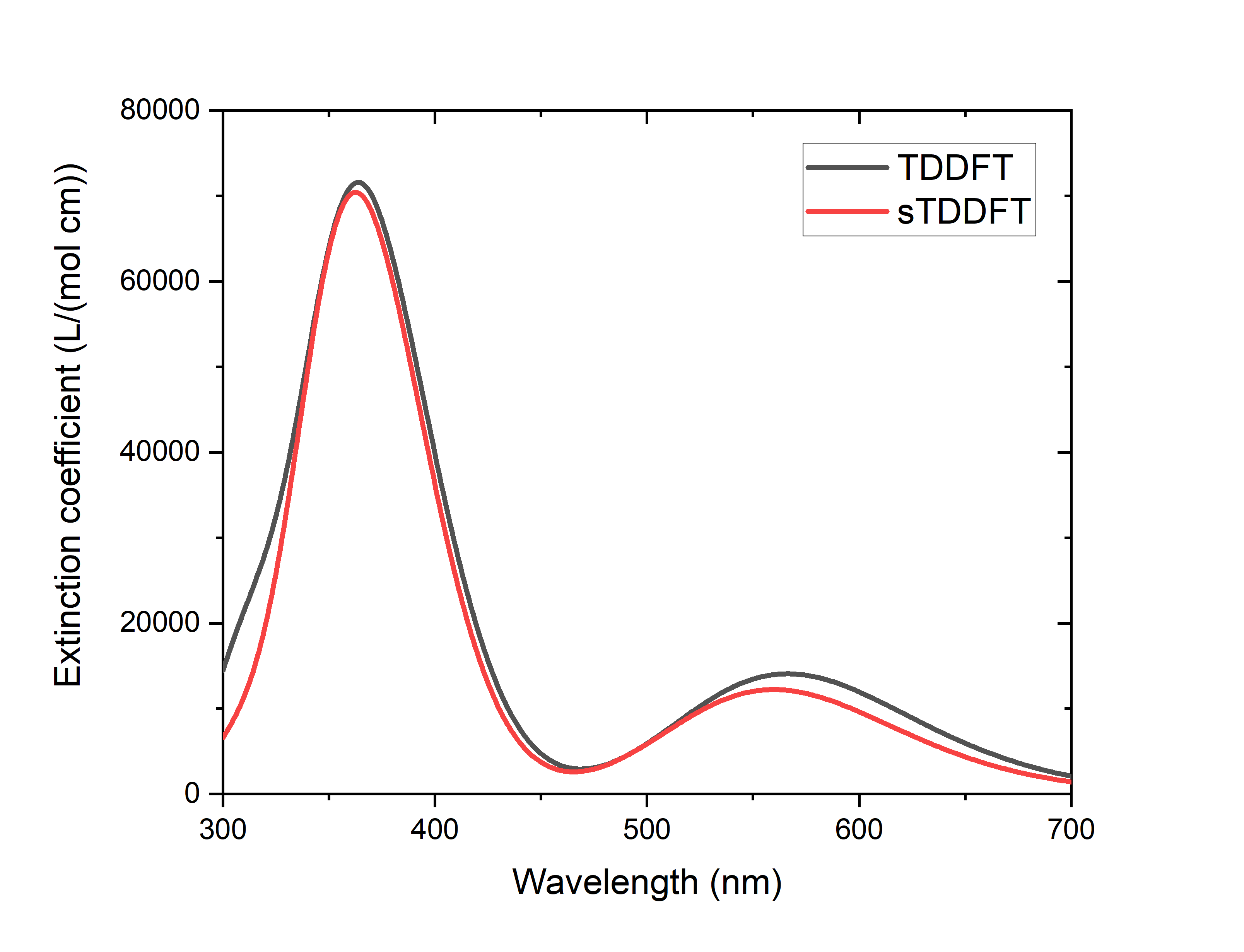
At the same time, sTDDFT saves 95% of the TDDFT calculation time compared with TDDFT (84% of the calculation time if the calculation time of SCF is included), which shows that the acceleration effect is very impressive.

In addition to sTDDFT, the grimmestd keyword can be used for TDA calculations to specify that sTDA calculations are performed, for example:

$tddft
Itda
 1
iwindow
 300 700 nm
grimmestd
$end

Of course, it is also possible to specify the number of excited states calculated instead of the wavelength range:

$tddft
nroot # calculate 100 lowest excited states per irrep
 100
grimmestd
$end

For more information, see Grimmestd Keyword Introduction <grimmestd>.

Restart the TDDFT task that was unexpectedly interrupted

If the TDDFT calculation is terminated unexpectedly, the user may want to reschedule the calculation, that is, when the TDDFT calculation is redone, some intermediate results generated by the previously interrupted TDDFT task are used to reduce or avoid redundant calculation. For details on how to calculate the breakpoint restart of TDDFT, see the corresponding introduction in the FAQ chapter <tddftrestart>.

Mapping of Gaussian broadened absorption spectra

The above calculations only obtain the excitation energy and oscillator intensity of each excited state, and the user often needs to obtain the peak shape of the absorption spectrum predicted theoretically, which requires the absorption of each excited state to be Gaussian broadened according to a certain half-peak width. In BDF, this is achieved via a Python script plotspec.py (located under $BDFHOME/sbin/, where $BDFHOME is the installation path of BDF). After the TDDFT calculation is completed, you need to manually invoke the plotspec.py from the command line. For example, if we have calculated the TDDFT excited state of the C60 molecule with BDF, and the corresponding output file is C60.out, we can run it

$BDFHOME/sbin/plotspec.py C60.out

or

$BDFHOME/sbin/plotspec.py C60

The script outputs the following information on the screen:

==================================
      P  L  O  T  S  P  E  C

 Spectral broadening tool for BDF
==================================

BDF output file: C60.out

1 TDDFT output block(s) found
Block 1: 10 excited state(s)
 - Singlet absorption spectrum, spin-allowed

The spectra will be Gaussian-broadened (FWHM = 0.5000 eV) ...

Absorption maxima of spectrum 1 (nm (lg epsilon/(L/(mol cm)))):
 - 238 (5.12), 308 (4.50)

plotspec.py: exit successfully

Two files are generated, one is C60.stick.csv, containing the absorption wavelengths and molar extinction coefficients of all excited states, which can be used as a bar plot:

TDDFT Singlets 1,,
Wavelength,Extinction coefficient,
nm,L/(mol cm),
867139,2899.779319,
302300,31192.802393,
635960,131840.430395,
765024,295.895849,
090150,134.498113,
019205,179194.526059,
561512,145.257962,
943322,54837.570677,
778366,548.752301,
167663,780.089056,

The other is C60.spec.csv, which contains the absorption spectrum after Gaussian broadening (the default broadening FWHM is 0.5 eV):

TDDFT Singlets 1,,
Wavelength,Extinction coefficient,
nm,L/(mol cm),
200.000000,162720.545118,
201.000000,151036.824457,
202.000000,137429.257570,
...
998.000000,0.000000,
999.000000,0.000000,
1000.000000,0.000000,

These two files can be opened and plotted with Excel, Origin, and other graphing software:

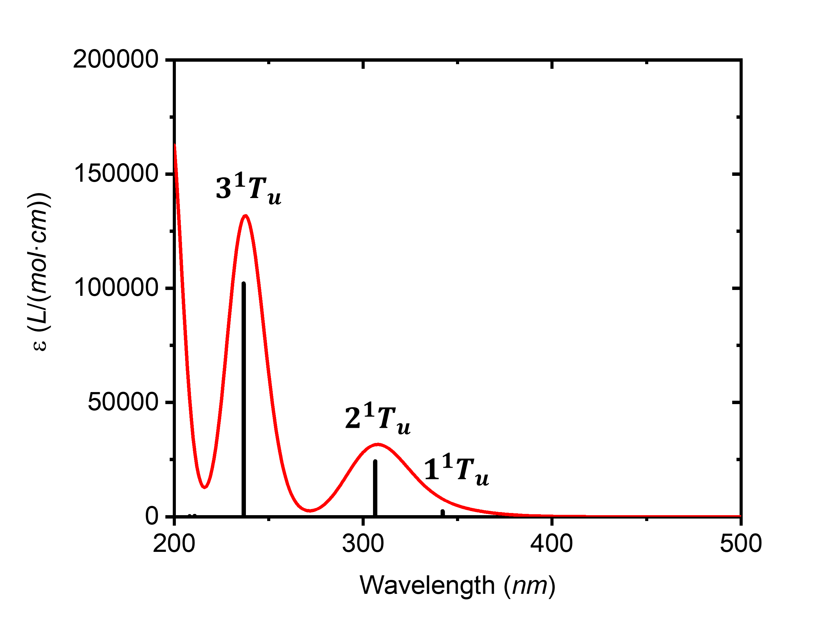
Command line arguments can be used to control the plotting range, Gaussian broadened FWHM, and so on. Example:

# Plot the spectrum in the range 300-600 nm:
 $BDFHOME/sbin/plotspec.py wavelength=300-600nm filename.out

# Plot an X-ray absorption spectrum in the range 200-210 eV,
# using an FWHM of 1 eV:
 $BDFHOME/sbin/plotspec.py energy=200-210eV fwhm=1eV filename.out

# Plot a UV-Vis spectrum in the range 10000 cm-1 to 40000 cm-1,
# where the wavenumber is sampled at an interval of 50 cm-1:
 $BDFHOME/sbin/plotspec.py wavenumber=10000-40000cm-1 interval=50 filename.out

# Plot an emission spectrum in the range 600-1200 nm, as would be
# given by Kasha's rule (i.e. only the first excited state is considered),
# where the wavelength is sampled at an interval of 5 nm:
 $BDFHOME/sbin/plotspec.py -emi wavelength=600-1200nm interval=5 filename.out

If you don’t run $BDFHOME/sbin/plotspec.py without command line arguments, you can list all command line arguments and usages, which will not be repeated here.

Calculation of electron circular dichroism (ECD) spectra

In addition to absorption spectra, BDF also supports the calculation of circular dichroism (ECD) spectra at TDDFT levels. The user only needs to add the ECD keyword to the input of the $tddft module. For example, the following input file calculates the ECD spectrum of (S)-5-methylcyclopenta-2-en-1-one in the range of 160-300 nm at the wB97X/ma-def2-TZVP level with water as solvent:

$COMPASS
Title
 ECD test
Basis
 ma-def2-TZVP
Geometry # B3LYP/def2-SVP geometry
  C   11.03017501307698     -1.06358915357097     18.65132535474617
  C   12.57384005718525     -1.02456284484694     18.65658561738920
  C   12.91529117412091      0.43177145174825     18.82255138315294
  C   11.83078974644673      1.23189442235475     18.82242608164620
  H   10.67388955940226     -1.47007769437446     19.61628109972719
  H   13.00096293117676     -1.40629079282790     17.71067917782706
  H   13.02306939327327     -1.63533989080155     19.45869631125239
  H   13.94838829748073      0.77963695466942     18.91842719115154
  H   11.81586135485978      2.32060314334658     18.90537981712256
  C   10.61010494985639      0.41685642111484     18.65633627754937
  O    9.46516754355473      0.82239910074197     18.54006339565965
  C   10.37591484801120     -1.85714650215417     17.51891751829459
  H   10.61141701850992     -2.93014535161767     17.59810807151853
  H    9.28153845878811     -1.73962079399751     17.55678289237466
  H   10.72376849425688     -1.50217177978463     16.53426564058783
End Geometry
MPEC+COSX
$END

$XUANYUAN
rs
 0.3
$END

$SCF
RKS
DFT
 wB97X
solvent
 water
Solmodel
 SMD # IEFPCM is also a reasonable choice and is almost equally accurate
$END

$tddft
iprt
 3
# To ensure that we get all roots within the window, we use the iVI method.
# Nevertheless, of course, iVI is not mandatory for ECD calculations
idiag
 3# use iVI
iwindow
 160 300 nm
ecd # specifies ECD calculation
solneqlr # linear response solvation, recommended when the number of excited states
         # is large
$end

After the output of the absorption wavelength, oscillator intensity, and transition dipole moment, the transition magnetic dipole moment, and the rotor strength under the length and velocity manifestations are also printed:

*** Ground to excited state Transition magnetic dipole moments (Au) ***
   State          X           Y           Z
  -0.001936     0.002882     0.000034
  -0.000444    -0.000188    -0.004692
  -0.000342    -0.003475    -0.000070
  -0.001232     0.000479    -0.001992
   0.000581     0.002272    -0.001047
  -0.001917     0.003593    -0.000178
   0.002065     0.000206    -0.000823


*** Electronic circular dichroism (ECD) rotatory strengths (1e-40 cgs) ***
   State      Length formalism     Velocity formalism
             -2.9144               -3.0791
             18.0007               17.5760
            -25.1038              -25.1132
             -7.2316               -7.0551
             25.1323               24.4034
            -14.9753              -14.2051
            -30.6305              -30.8057

Next, you can use plotspec.py to read the rotor intensity information in the output file, perform Gaussian broadening, and obtain .spec.csv and .stick.csv files to make ECD plots (where the excited states with an absorption wavelength slightly less than 160 nm will have a certain impact on the spectra around 160 nm after Gaussian broadening, and the ECD spectra near 160 nm may not be reliable, so only 180 nm can be used for mapping):

$BDFHOME/sbin/plotspec.py -cd wavelength=180-300 filename.out

Here are the results:

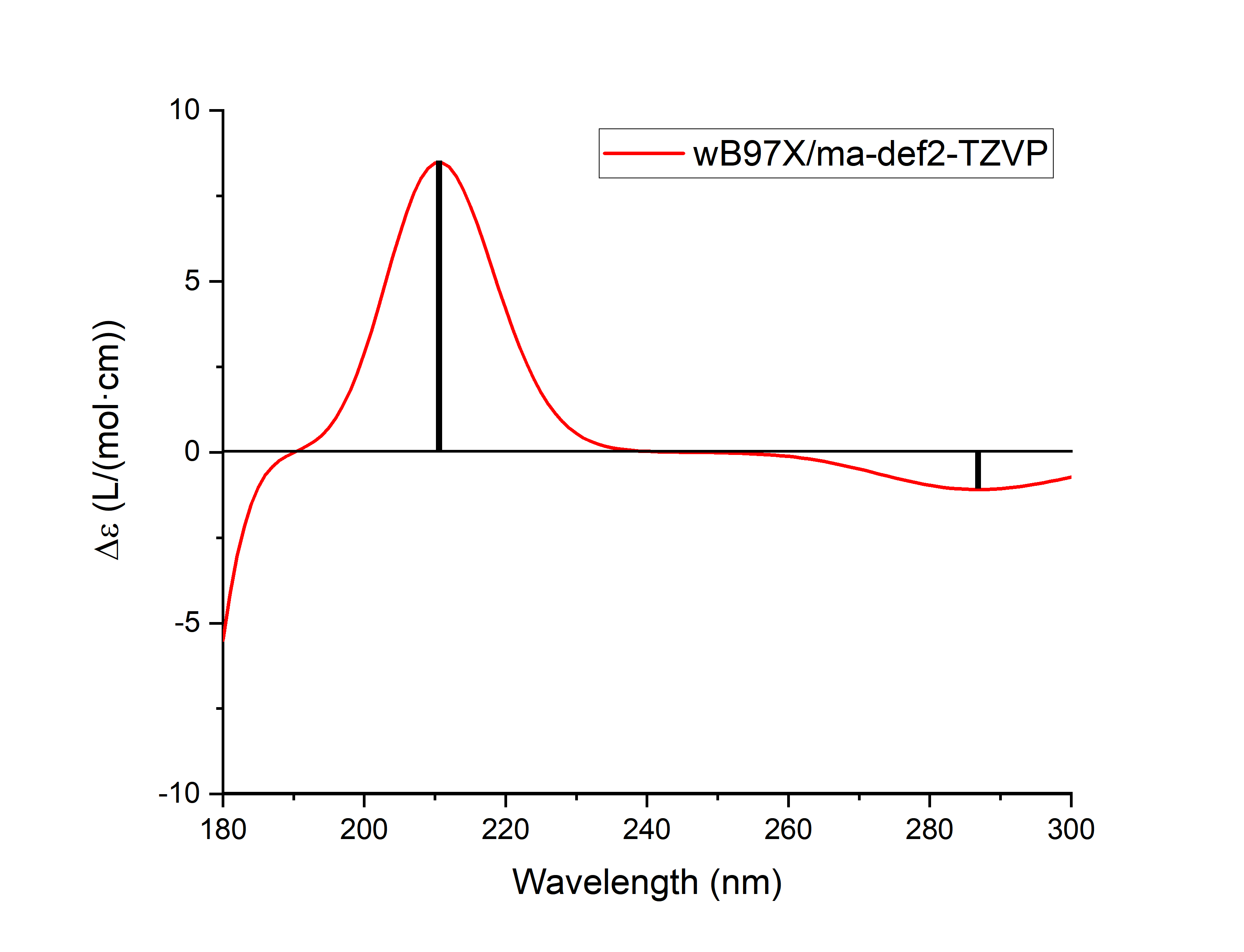
Note

Although the rotor strength under the velocity gauge and the rotor strength under the length gauge are strictly equal when the basis set tends to be complete, when the size of the basis set is limited, the rotor strength under the velocity gauge does not depend on the orientation and center position of the molecule, but the rotor strength under the length gauge is dependent on the orientation and center position of the molecule. Therefore, at least when the molecule is relatively large and the basis set is not too large, the rotor strength results under the velocity gauge are more reliable. plotspec.py by default, the ECD diagram is plotted with the rotor strength under the velocity gauge, if you need to use the rotor strength under the length gauge to plot the ECD diagram, you should change the -cd in the command line argument of the plotspec.py to -cdl.
Due to the difference between BDF and other programs to determine the molecular standard orientation and the origin of molecular coordinates, the rotor strength calculated by BDF under the length representation may be slightly different from other programs, which is a normal phenomenon and is caused by the theoretical defects of the rotor strength under the above length gauge, and does not mean that the calculation results are wrong. However, the rotor strength under the velocity gauge should be in good agreement with other procedures.
For flexible molecules, the ECD calculation results of a single conformation are not reliable, it is recommended to combine CREST, Molclus and other software to perform conformational search, calculate the ECD spectra for all major conformations separately, and then perform Boltzmann weighted average.

Optimization of excited state structure

BDF not only supports the calculation of TDDFT single-point energy (i.e., the excitation energy under a given molecular structure), but also supports the structural optimization and numerical frequency calculation of the excited state. To do this, it is necessary to add the $resp module after the $tddft module to calculate the gradient of TDDFT energy, and the $bdfopt module after the $compass module to use the TDDFT gradient information for structure optimization and frequency calculation (see GeomOptimization<> for details).

The following is an example of optimizing the structure of the first excited state of butadiene at the B3LYP/cc-pVDZ level:

$COMPASS
Title
 C4H6
Basis
 CC-PVDZ
Geometry # Coordinates in Angstrom. The structure has C(2h) symmetry
 C -1.85874726  -0.13257980  0.00000000
 H -1.95342119  -1.19838319  0.00000000
 H -2.73563916   0.48057645  0.00000000
 C -0.63203020   0.44338226  0.00000000
 H -0.53735627   1.50918564  0.00000000
 C  0.63203020  -0.44338226  0.00000000
 H  0.53735627  -1.50918564  0.00000000
 C  1.85874726   0.13257980  0.00000000
 H  1.95342119   1.19838319  0.00000000
 H  2.73563916  -0.48057645  0.00000000
End Geometry
$END

$BDFOPT
solver
 1
$END

$XUANYUAN
$END

$SCF
RKS
dft
 B3lyp
$END

$TDDFT
nroot
# The ordering of irreps of the C(2h) group is: Ag, Au, Bg, Bu
# Thus the following line specifies the calculation of the 1Bu state, which
# happens to be the first excited state for this particular molecule.
 0 0 0 1
istore
 1
# TDDFT gradient requires tighter TDDFT convergence criteria than single-point
# TDDFT calculations, thus we tighten the convergence criteria below.
crit_vec
 1.d-6 # default 1.d-5
crit_e
 1.d-8 # default 1.d-7
$END

$resp
Geom
norder
 1 # first-order nuclear derivative
method
 2 # TDDFT response properties
nfiles
 1 # must be the same number as the number after the istore keyword in $TDDFT
iroot
 1 # calculate the gradient of the first root. Can be omitted here since only
   # one root is calculated in the $TDDFT block
$end

Note that in the above example, the meaning of the keyword ‘’iroot’’ in the ‘’$resp’’ module is different from the keyword ‘’’iroot’’ in the ‘’$tddft’’ module. The former refers to the calculation of the gradient of the first few excited states, while the latter refers to the number of excited states that are calculated in total for each irreducible representation.

After the molecular structure is optimized and converged, the converged structure is output in the main output file:

 Good Job, Geometry Optimization converged in     5 iterations!

Molecular Cartesian Coordinates (X,Y,Z) in Angstrom :
   C          -1.92180514       0.07448476       0.00000000
   H          -2.21141426      -0.98128927       0.00000000
   H          -2.70870517       0.83126705       0.00000000
   C          -0.54269837       0.45145649       0.00000000
   H          -0.31040658       1.52367715       0.00000000
   C           0.54269837      -0.45145649       0.00000000
   H           0.31040658      -1.52367715       0.00000000
   C           1.92180514      -0.07448476       0.00000000
   H           2.21141426       0.98128927       0.00000000
   H           2.70870517      -0.83126705       0.00000000

                    Force-RMS    Force-Max     Step-RMS     Step-Max
 Conv. tolerance :  0.2000E-03   0.3000E-03   0.8000E-03   0.1200E-02
 Current values  :  0.5550E-04   0.1545E-03   0.3473E-03   0.1127E-02
 Geom. converge  :     Yes          Yes          Yes          Yes

In addition, the excitation energy under the excited state equilibrium structure, as well as the total energy and main components of the excited state, can be read from the output of the last TDDFT module of the .out.tmp file:

 Well.     1 w= 5.1695 eV -155.6874121542 a.u.  f= 0.6576 D<Pab>= 0.0000 Ova= 0.8744
      CV(0): Ag( 6 )-> Bu( 10 ) c_i: 0.1224 Per: 1.5% IPA: 17.551 eV Oai: 0.6168
      CV(0): Bg( 1 )-> Au( 2 ) c_i: -0.9479 Per: 89.9% IPA: 4.574 eV Oai: 0.9035

...

  No. Pair   ExSym   ExEnergies  Wavelengths      f     D<S^2>          Dominant Excitations             IPA   Ova     En-E1

    1 Bu 1 Bu 5.1695 eV 239.84 nm 0.6576 0.0000 89.9% CV(0): Bg( 1 )-> Au( 2 ) 4.574 0.874 0.0000

Among them, the wavelength corresponding to the excitation energy under the excited state equilibrium structure (240 nm) is the fluorescence emission wavelength of butadiene.

Note

The optimized excited state structure of some systems will oscillate without convergence, which is generally due to the optimization near the conical intersection. If the optimization is near the conical intersection of the excited state and the ground state, and full TDDFT is used instead of TDA, the structure optimization may even be error-exited due to the excitation energy becoming imaginary or complex. These two situations are normal, and the causes and solutions are detailed in Geometric Optimization Non-Convergent Solution <geomoptnotconverged>.

Spin-orbit coupling calculation based on sf-X2C/TDDFT-SOC

Relativistic effects include scalar relativity and spin-orbit coupling (SOC). Relativistic calculations require the use of a basis set optimized for relativistic effects, and choose the right Hamiltonian**. BDF supports all-electron sf-X2C/TDDFT-SOC calculations, where sf-X2C refers to the consideration of scalar relativistic effects by Hamiltonian of an exact two-component (X2C) without spin, and TDDFT-SOC refers to the calculation of spin-orbit coupling based on TDDFT. Note that although TDDFT is an excited state method, TDDFT-SOC can be used to calculate the contribution of SOC not only to the energy and properties of the excited state, but also to calculate the contribution of SOC to the energy and properties of the ground state.

Taking a molecule with a ground state as a singlet as an example, the sf-X2C/TDDFT-SOC calculation needs to call TDDFT three times in order to complete the calculation. Among them, the first calculation uses R-TDDFT to compute the singlet state, The second time the triplet state was calculated by SF-TDDFT, and wave functions calculated by the first two TDDFT was read in for the last time, and the state interaction (SI) method was used to calculate the spin-orbit couplings for these states. This is clearly seen from the advanced inputs for the sf-X2C/TDDFT-SOC calculation for the :math:’ce{CH2S}’ molecule below.

$COMPASS
Title
 ch2s
Basis # Notice: we use relativistic basis set contracted by DKH2
  cc-pVDZ-DK
Geometry
C       0.000000    0.000000   -1.039839
S       0.000000    0.000000    0.593284
H       0.000000    0.932612   -1.626759
H       0.000000   -0.932612   -1.626759
End geometry
$END

$xuanyuan
heff  # ask for sf-X2C Hamiltonian
 3
hsoc  # set SOC integral as 1e+mf-2e
 2
$end

$scf
RKS
dft
  PBE0
$end

#1st: R-TDDFT, calculate singlets
$tddft
ISF
 0
idiag
 1
iroot
 10
Itda
 0
istore # save TDDFT wave function in the 1st scratch file
 1
$end

#2nd: spin-flip tddft, use close-shell determinant as reference to calculate triplets
$tddft
isf # notice here: ask for spin-flip up calculation
 1
Itda
 0
idiag
 1
iroot
 10
istore # save TDDFT wave function in the 2nd scratch file, must be specified
 2
$end

#3rd: tddft-soc calculation
$tddft
isoc
 2
nprt # print level
 10
nfiles
 2
ifgs # whether to include the ground state in the SOC treatment. 0=no, 1=yes
 1
imatsoc
 8
 0 0 0 2 1 1
 0 0 0 2 2 1
 0 0 0 2 3 1
 0 0 0 2 4 1
 1 1 1 2 1 1
 1 1 1 2 2 1
 1 1 1 2 3 1
 1 1 1 2 4 1
imatrso
 6
 1 1
 1 2
 1 3
 1 4
 1 5
 1 6
idiag # full diagonalization of SO Hamiltonian
 2
$end

Warning

Calculations must be performed in the order of isf=0, isf=1. When the SOC treatment does not consider the ground state (i.e., ‘’ifgs=0’’), the more excited states ‘’iroot’’’ are calculated, the more accurate the result is; When considering the ground state (i.e., ‘’ifgs=1’’’), too much ‘’iroot’’ will reduce the accuracy, which is manifested in the underestimation of the ground state energy.

The keyword imatsoc controls which SOC matrix elements $<A|hso|B>$ to be printed,

‘’8’’ means that you want to print SOC between 8 sets of spinor states, and 8 lines of integer arrays are entered in the following order;

The input format for each line is fileA symA stateA fileB symB stateB, which represents the matrix elements <fileA,symA,stateA|hsoc|fileB,symB,stateB>, where

fileA symA stateA represents the irreducible root of stateA in file fileA; For example, ‘’1 1 1’’ represents the 1st root of the 1st irreducible representation calculated by the 1st TDDFT;

‘’0 0 0’’ denotes the ground state

Note

The program can only print a maximum of 4000 SOC matrix elements at a time.

The printout of the coupling matrix element is as follows,

  [tddft_soc_matsoc]

Print selected matrix elements of [Hsoc]

SocPairNo. =    1   SOCmat = <  0  0  0 |Hso|  2  1  1 >     Dim =    1    3
  mi/mj ReHso(au) cm^-1 ImHso(au) cm^-1
 0.0 -1.0      0.0000000000      0.0000000000      0.0000000000      0.0000000000
 0.0  0.0      0.0000000000      0.0000000000      0.0000000000      0.0000000000
 0.0  1.0      0.0000000000      0.0000000000      0.0000000000      0.0000000000

SocPairNo. =    2   SOCmat = <  0  0  0 |Hso|  2  2  1 >     Dim =    1    3
  mi/mj ReHso(au) cm^-1 ImHso(au) cm^-1
 0.0 -1.0      0.0000000000      0.0000000000      0.0000000000      0.0000000000
 0.0  0.0      0.0000000000      0.0000000000      0.0007155424    157.0434003237
 0.0  1.0      0.0000000000      0.0000000000     -0.0000000000     -0.0000000000

SocPairNo. =    3   SOCmat = <  0  0  0 |Hso|  2  3  1 >     Dim =    1    3
  mi/mj ReHso(au) cm^-1 ImHso(au) cm^-1
 0.0 -1.0     -0.0003065905    -67.2888361761      0.0000000000      0.0000000000
 0.0  0.0      0.0000000000      0.0000000000     -0.0000000000     -0.0000000000
 0.0  1.0     -0.0003065905    -67.2888361761     -0.0000000000     -0.0000000000

Here, ‘’< 0 0 0 | Hso| 2 2 1 >’’ represents the matrix element ‘’<S0| Hso| T1>’’ , giving the actual part ReHso and the imaginary part ImHso, respectively. Since S0 has only one component, mi is 0. T1 (spin S=1) has 3 components (Ms=-1,0,1), and these 3 components are numbered by mj. where the component of ‘’Ms=0’’ is coupled with the ground state, and the imaginary part of the matrix element is ‘’0.0007155424 au’’.

Warning

When comparing the results of different programs, it is important to note that the so-called spherical tensor is given here, not the cartesian tensor, i.e. T1 is T_{-1}, T_{0}, T_{1}, not Tx, Ty, Tz, and there is a unitary transformation between the two.

The SOC is calculated as follows,

     Totol No. of States:   161  Print:    10

 In.     1 w= -0.0006 eV
      Spin: |Gs,1>    1-th Spatial:  A1;  OmegaSF=      0.0000eV  Cr=  0.0000  Ci=  0.9999  Per:100.0%
    SumPer: 100.0%

 In.     2 w= 1.5481 eV
      Spin: |S+,1>    1-th Spatial:  A2;  OmegaSF=      1.5485eV  Cr=  0.9998  Ci= -0.0000  Per:100.0%
    SumPer: 100.0%

 In.     3 w= 1.5482 eV
      Spin: |S+,3>    1-th Spatial:  A2;  OmegaSF=      1.5485eV  Cr=  0.9998  Ci=  0.0000  Per:100.0%
    SumPer: 100.0%

 In.     4 w= 1.5486 eV
      Spin: |S+,2>    1-th Spatial:  A2;  OmegaSF=      1.5485eV  Cr=  0.9999  Ci=  0.0000  Per:100.0%
    SumPer: 100.0%

 In.     5 w= 2.2106 eV
      Spin: |So,1>    1-th Spatial:  A2;  OmegaSF=      2.2117eV  Cr= -0.9985  Ci=  0.0000  Per: 99.7%
    SumPer:  99.7%

 In.     6 w= 2.5233 eV
      Spin: |S+,1>    1-th Spatial:  A1;  OmegaSF=      2.5232eV  Cr=  0.9998  Ci=  0.0000  Per:100.0%
    SumPer: 100.0%

 In.     7 w= 2.5234 eV
      Spin: |S+,3>    1-th Spatial:  A1;  OmegaSF=      2.5232eV  Cr=  0.9998  Ci= -0.0000  Per:100.0%
    SumPer: 100.0%

 In.     8 w= 2.5240 eV
      Spin: |S+,2>    1-th Spatial:  A1;  OmegaSF=      2.5232eV  Cr=  0.0000  Ci= -0.9985  Per: 99.7%
    SumPer:  99.7%

 In.     9 w= 5.5113 eV
      Spin: |S+,1>    1-th Spatial:  B2;  OmegaSF=      5.5115eV  Cr= -0.7070  Ci= -0.0000  Per: 50.0%
      Spin: |S+,3>    1-th Spatial:  B2;  OmegaSF=      5.5115eV  Cr=  0.7070  Ci=  0.0000  Per: 50.0%
    SumPer: 100.0%

 In.    10 w= 5.5116 eV
      Spin: |S+,1>    1-th Spatial:  B2;  OmegaSF=      5.5115eV  Cr= -0.5011  Ci= -0.0063  Per: 25.1%
      Spin: |S+,2>    1-th Spatial:  B2;  OmegaSF=      5.5115eV  Cr=  0.7055  Ci=  0.0000  Per: 49.8%
      Spin: |S+,3>    1-th Spatial:  B2;  OmegaSF=      5.5115eV  Cr= -0.5011  Ci= -0.0063  Per: 25.1%
    SumPer: 100.0%

*** List of SOC-SI results ***

 No.      ExEnergies Dominant Excitations Esf dE Eex(eV) (cm^-1)

   1      -0.0006 eV   100.0%  Spin: |Gs,1>    0-th   A1    0.0000   -0.0006    0.0000         0.00
   2       1.5481 eV   100.0%  Spin: |S+,1>    1-th   A2    1.5485   -0.0004    1.5487     12491.27
   3       1.5482 eV   100.0%  Spin: |S+,3>    1-th   A2    1.5485   -0.0004    1.5487     12491.38
   4       1.5486 eV   100.0%  Spin: |S+,2>    1-th   A2    1.5485    0.0001    1.5492     12494.98
   5       2.2106 eV    99.7%  Spin: |So,1>    1-th   A2    2.2117   -0.0011    2.2112     17834.44
   6       2.5233 eV   100.0%  Spin: |S+,1>    1-th   A1    2.5232    0.0002    2.5239     20356.82
   7       2.5234 eV   100.0%  Spin: |S+,3>    1-th   A1    2.5232    0.0002    2.5239     20356.99
   8       2.5240 eV    99.7%  Spin: |S+,2>    1-th   A1    2.5232    0.0008    2.5246     20362.08
   9       5.5113 eV    50.0%  Spin: |S+,1>    1-th   B2    5.5115   -0.0002    5.5119     44456.48
  10       5.5116 eV    49.8%  Spin: |S+,2>    1-th   B2    5.5115    0.0001    5.5122     44458.63

The output here has two parts, the first part gives the energy and composition of each SOC-SI state with respect to the S0 state, for example

``No. 10 w= 5.5116 eV’’ means that the energy of the 10th ‘’SOC-SI’’’ state is ‘’5.5116 eV’’, note that here is the energy relative to the S0 state;

The following three lines are the components of this state,

``Spin: | S+,1> 1-th Spatial: B2; ‘’ means that this is the first triplet state with symmetry of B2 (with respect to the S-state spin +1, and therefore S+);

‘’OmegaSF= 5.5115eV’’ is the energy relative to the first spinor state;

‘’Cr= -0.5011 Ci= -0.0063’’ is the real and imaginary part of the wave function of this component in the spinor state, and the percentage is ‘’25.1%’’.

The second part summarizes the results of the SOC-SI states.

ExEnergies lists the excitation energy after considering the SOC. ‘’Esf’’ is the excitation energy when the original SOC is not considered; * The excited state is expressed with ‘’Spin: | S,M> n-th sym’’ to denote spin | Gs, 1>, the spatial symmetry is the nth state of sym. For example, | Gs,1> represents the ground state, | So,1> represents the excited state in which the total spin and ground state are the same, | S+,2> represents the excited state of the total spin plus 1. M is the component of the spin projection (in total 2S+1).

The keyword ‘’imatrso’’ specifies which sets of transition dipole moments between spinor states to be calculated and printed. Here it is specified to print the ‘’6’’ group of transition dipole moments,

‘’1 1’’ denotes the ground state intrinsic dipole moment;

‘’1 2’’ denotes the transition dipole moment between the first and second spinor states.

Note

The program can only print up to 4000 sets of transition dipole moments at a time.

The output of the transition dipole moment is as follows:

[tddft_soc_matrso]: Print selected matrix elements of [dpl]

 No.  ( I , J ) |rij|^2 E_J-E_I fosc rate(s^-1)
-------------------------------------------------------------------------------
  1 1 1 0.472E+00 0.0000000000 0.0000000000 0.000E+00
  Details of transition dipole moment with SOC (in a.u.):
                  <I|X|J>       <I|Y|J>       <I|Z|J>        (also in debye)
         Real= -0.113E-15 -0.828E-18 0.687E+00 -0.0000 -0.0000 1.7471
         Imag=  -0.203E-35     0.948E-35     0.737E-35    -0.0000   0.0000   0.0000
         Norm=   0.113E-15     0.828E-18     0.687E+00



 No.  ( I , J ) |rij|^2 E_J-E_I fosc rate(s^-1)
-------------------------------------------------------------------------------
  2 1 2 0.249E-05 1.548720567 0.000000095 0.985E+01
  Details of transition dipole moment with SOC (in a.u.):
                  <I|X|J>       <I|Y|J>       <I|Z|J>        (also in debye)
         Real= -0.589E-03 0.207E-07 -0.177E-15 -0.0015 0.0000 -0.0000
         Imag=  -0.835E-08     0.147E-02    -0.198E-16    -0.0000   0.0037  -0.0000
         Norm=   0.589E-03     0.147E-02     0.178E-15

Hint

imatsoc is set to -1 to specify that all coupling matrix elements are printed;
By default, the transition dipole moment is not calculated, and the transition dipole moment between all spinor states can be printed by setting imatrso to ‘’-1’’, and the transition dipole moment between all ground spinor states and all excited spinor states can be printed by setting imatrso to ‘’-2’’.
The reference state of the SOC calculation must be either RHF/RKS or ROHF/ROKS, UHF/UKS is not supported.
When the reference state of the SOC calculation is ROHF/ROKS, the TDDFT calculation of isf=0 must use X-TDA (i.e., itest=1, icorrect=1, isf=0, itda=1; full X-TDDFT is not supported), and the TDDFT calculation of isf=1 must use SF-TDA (i.e., isf=1, itda=1; full SF-TDDFT is not supported).

TDDFT-SOC spin-orbit coupling calculation using ECP base set

In addition to the sf-X2C all-electron scalar relativistic Hamiltonian, the pseudopotential can also be used for TDDFT-SOC spin-orbit coupling calculations, in which the spin-orbit coupling pseudopotential (SOECP) is the first choice. To do this, you need to select the appropriate spin-orbit-coupled Pseudopotential Basis Set <soecp-bas> and set the hsoc to 10 in the Xuanyuan module (you can also write other values, But it will be treated as 10). Other inputs are similar or identical to the sf-X2C/TDDFT-SOC inputs (e.g. core electrons are excluded when specifying orbital occupancy in ‘’scf’’).

In the example below, the closed-shell ground state of the InBr molecule is calculated under the symmetry of the :math:’C_{2v}’ point group, and the lowest three excited states of the InBr molecule :math:’^3Pi’ (B1+B2), :math:’^1Pi’ (B1+B2), :math:’^3Sigma^+’ (A1), where the first two Λ-S states are bound states that have been extensively experimentally studied, THE LAST TWO Λ-S STATES ARE REPULSIVE STATES AND ARE NOT MUCH OF AN EXPERIMENTAL CONCERN. In the input, the energy of the Λ-S state is calculated and the wave function is stored at the TDDFT level (Tamm-Dancoff approximation is used here), and then the energy of the Ω state after spin-orbit coupling is calculated.

$COMPASS
Title
 soecp test: InBr
Basis-block
  cc-pVTZ-PP
end basis
Geometry
  In  0.0  0.0  0.0
  Br  0.0  0.0  2.45
END geometry
group
 C(2v)      # Abelian symmetry must be used for SOC
$END

$XUANYUAN
 hsoc
  10
$END

$scf
  rks
  dft
   pbe0
$end

$TDDFT
ISF
 0
ITDA
 1
istore
 1
# 1Pi state: A1, A2, B1, B2
nroot
  0 0 1 1
$END

$TDDFT
ISF
 1
ITDA
 1
istore
 2
# 3Sigma+ and 3Pi states: A1, A2, B1, B2
nroot
  1 0 1 1
$END

$TDDFT
isoc
 2
nfiles
 2
ifgs
 1
idiag
 2
$END

The calculated output of SOECP/TDFT-SOC is similar to that of the sf-X2C/TDDFT-SOC. The results are summarized below and compared to those of the two-component EOM-CCSD.

L-S state | TDDFT | Ω state | TDDFT-SOC | Splitting Energy | Two-Component EOM-CCSD | Splitting Energy | +=====================+=============+=====+=============+=============+==============+=============+ | :math:’X^1Sigma^+’ | 0 | 0+ | 0 | | 0 | | +———————+————-+—–+————-+————-+————–+————-+ | :math:’^3Pi’ | 25731 | 0- | 24884 | | 24516 | | +———————+————-+—–+————-+————-+————–+————-+ | | | 0+ | 24959 | 75 | 24588 | 72 | +———————+————-+—–+————-+————-+————–+————-+ | | | 1 | 25718 | 759 | 25363 | 775 | +———————+————-+—–+————-+————-+————–+————-+ | | | 2 | 26666 | 948 | 26347 | 984 | +———————+————-+—–+————-+————-+————–+————-+ | :math:’^1Pi’ | 35400 | 1 | 35404 | | 36389 | | +———————+————-+—–+————-+————-+————–+————-+ | :math:’^3Sigma^+’ | 38251 | 0- | 38325 | | | | +———————+————-+—–+————-+————-+————–+————-+ | | | 1 | 38423 | 98 | | | +———————+————-+—–+————-+————-+————–+————-+

In addition to the SOECP basis set, the above calculation can also be done with a scalar ECP basis set combined with the effective nuclear charge approximation (Zeff) <so1e-zeff>’. As a test, first remove the SO pseudopotential part of the Br basis set and redo the above calculation, but you will find that the results are poor: The split between :math:’^3Pi_2’ and :math:’^3Pi_1’ is only 850 cm :math:’^{-1}’, while the split between :math:’^3Sigma^+’ is almost zero. This is because the ECP base set of Br with 10 cores does not have a specially optimized effective nuclear charge, and the program can only take the actual number of nuclear charges 35:

SO-1e[BP]
          Zeff for Wso
----------------------------------
 IAtm     ZA    NCore         Zeff
----------------------------------
    1     49       28        SOECP
    2 35 10 N.A.
----------------------------------

For Br in the above example, you may wish to use the scalar ECP base set cc-pVTZ-ccECP with 28 core electrons instead, and the input part of the basis set is modified as follows:

Basis-block
  cc-pvtz-pp
  Br=cc-pvtz-ccecp
end basis

Track occupancy is not specified in modules after xuanyuan, so there is no need to modify the input. It can be seen at the beginning of the TDDFT-SOC calculation output

SO-1e[BP]
          Zeff for Wso
----------------------------------
 IAtm     ZA    NCore         Zeff
----------------------------------
    1     49       28        SOECP
    2     35       28     1435.000
----------------------------------

This shows that in the single-electron spin-orbit integral of Br, the default nuclear charge number 35 is replaced with an optimized 1435.000 (in general, the larger the ECP core electron number NCore, the larger the effective nuclear charge Zeff), SOECP integrals are still calculated for the In atom. The results are as follows, and it can be seen that the SOC splitting has been significantly improved:

L-S state | TDDFT | Ω state | Br:SOECP | Splitting | Br:ECP | Splitting | +=====================+=============+=====+=============+=============+=============+=============+ | :math:’X^1Sigma^+’ | 0 | 0+ | 0 | | 0 | | +———————+————-+—–+————-+————-+————-+————-+ | :math:’^3Pi’ | 25731 | 0- | 24884 | | 25019 | | +———————+————-+—–+————-+————-+————-+————-+ | | | 0+ | 24959 | 75 | 25084 | 65 | +———————+————-+—–+————-+————-+————-+————-+ | | | 1 | 25718 | 759 | 25856 | 772 | +———————+————-+—–+————-+————-+————-+————-+ | | | 2 | 26666 | 948 | 26808 | 952 | +———————+————-+—–+————-+————-+————-+————-+ | :math:’^1Pi’ | 35400 | 1 | 35404 | | 35729 | | +———————+————-+—–+————-+————-+————-+————-+ | :math:’^3Sigma^+’ | 38251 | 0- | 38325 | | 38788 | | +———————+————-+—–+————-+————-+————-+————-+ | | | 1 | 38423 | 98 | 38853 | 65 | +———————+————-+—–+————-+————-+————-+————-+

Finally, TDDFT-SOC calculations can also be combined with SOECP (or scalar ECP) basis sets with all-electron non-relativistic basis sets. The BDF program has optimized Zeff for the all-electron non-relativistic basis set of the main group elements prior to Xe (except for the heavier noble gas elements). For example, if you continue to use cc-pVTZ-PP for In, and cc-pVTZ for Br, you will get similar results to SOECP/TDDFT-SOC. Detailed results omitted.

Attention

Precautions when using the effective nuclear charge method for TDDFT-SOC calculations: Optimized effective nuclear charge <SO1e-zeff>’ must be used to ensure accuracy. To do this, check the Zeff value printed in the output file and try not to show N.A., which is especially important for the ECP baseset.
Notes on all-electron basis sets when combining SOECP or scalar ECP with all-electron basis groups: Since atoms using all-electron basis sets do not consider scalar relativistic correspondence, they cannot be heavy atoms, and non-relativistic basis sets must be used.

Calculation of the first-order non-adiabatic coupled matrix element (fo-NACME).

As mentioned earlier, (first-order) non-adiabatic coupling matrix elements are of great significance in the non-radiative transition process, and one of their main uses is to calculate the internal convension rate constant (see azulene-example> for calculating the internal convension rate constant with BDF-MOMAP< ). In BDF, there are some differences in how the NACME input files between the ground state and the excited state, and between the excited state and the excited state are written separately.

Note

NACME between ground state and excited state, and NACME between excited state and excited state support R-TDDFT and U-TDDFT, but X-TDDFT is not supported.

NACME between ground state and excited state: :math:’ce{NO3}’ radical D0/D1 NACME (GB3LYP/cc-pVDZ)

$COMPASS
Title
 NO3 radical NAC, 1st excited state
Basis
 cc-pvdz
Geometry
N 0.00000000000 0.0000000000 -0.1945736441
O             -2.0700698389         0.0000000000        -1.1615808530
O              2.0700698389        -0.0000000000        -1.1615808530
O             -0.0000000000         0.0000000000         2.4934136445
End geometry
unit
 bohr
$END

$XUANYUAN
$END

$SCF
DOOR
dft
 GB3LYP
spinmulti
 2
$END

$tddft
iroot
 1 # One root for each irrep
istore
 1 # File number, to be used later in $resp
crit_vec
 1.d-6
crit_e
 1.d-8
gridtol
 1.d-7 # tighten the tolerance value of XC grid generation. This helps to
       # reduce numerical error, and is recommended for open-shell molecules
$end

$resp
iprt
 1
QUAD # quadratic response
FNAC # first-order NACME
single # calculation of properties from single residues (ground state-excited
       # state fo-NACMEs belong to this kind of properties)
norder
 1
method
 2
nfiles
 1 # must be the same as the istore value in the $TDDFT block
states
 1 # Number of excited states for which NAC is requested.
# First number 1: read TDDFT results from file No. 1
# Second number 2: the second irrep, in this case A2
#   (note: this is the pair symmetry of the particle-hole pair, not
#   the excited state symmetry. One must bear this in mind because the
#   ground state of radicals frequently does not belong to the totally
#   symmetric irrep)
#   If no symmetry is used, simply use 1.
# Third number 1: the 1st excited state that belongs to this irrep
 1 2 1
$end

Note: The irreducible representation specified in the $resp module is a pair irrep (i.e., the direct product of the irreducible representation of the occupied and empty orbits involved in the transition; For abelian point groups, pair irrep can be obtained from the direct product of the irreducible representation of the ground state and the irreducible representation of the excited state), but not the irrep of the excited state. The ground state (D0) of the molecule belongs to the B1 irreducible representation, and the first binary excited state (D1) belongs to the B2 irreducible representation, so the pair irrep of the D1 state is the direct product of B1 and B2, i.e., A2. Pair irrep can also be read from the output of the TDDFT module, i.e. in the Pair column of the following output sections:

No. Pair   ExSym   ExEnergies  Wavelengths      f     D<S^2>          Dominant Excitations             IPA   Ova     En-E1

A2 1 B2 0.8005 eV 1548.84 nm 0.0000 0.0186 98.2% CO(bb): B2( 2 )-> B1( 5 ) 3.992 0.622 0.0000
B1 1 A1 1.9700 eV 629.35 nm 0.0011 0.0399 92.2% CO(bb): A1(8)-> B1(5) 3.958 0.667 1.1695
B2 1 A2 2.5146 eV 493.06 nm 0.0000 0.0384 98.4% CO(bb): A2(1)-> B1(5) 4.159 0.319 1.7141
A1 2 B1 2.6054 eV 475.87 nm 0.0171 0.0154 87.7% CO(bb): B1( 4 )-> B1( 5 ) 3.984 0.746 1.8049

After the calculation is completed, at the end of the output section of the $resp module, you can see the result of the NACME calculation:

Gradient contribution from Final-NAC(R)-Escaled
      0.0000000000       -0.0000000000        0.0000000000
     -0.0000000000       -0.1902838724        0.0000000000
     -0.0000000000        0.1902838724        0.0000000000
     -0.0000000000        0.0000000000        0.0000000000

It can be found that the calculation results have N rows (where N is the number of atoms of the system), and each row has 3 real numbers, representing the x, y, and z components of the NACME of the atoms. Note that this result does not include the contribution of the electron translation factor (ETF), and for some molecules, NACME excluding ETF may not have translational invariance, which may lead to errors in subsequent calculations such as kinetic simulations. In this case, you need to use NACME with ETF in mind, which can be read later in the output file:

Gradient contribution from Final-NAC(S)-Escaled
      0.0000000000       -0.0000000000        0.0000000000
     -0.0000000000       -0.1920053581        0.0000000000
     -0.0000000000        0.1920053581        0.0000000000
     -0.0000000000        0.0000000000       -0.0000000000

The program also outputs vectors named dpq-R, Final-NAC(R), dpq-S, Final-NAC(S), etc., which are intermediate variables and are only used to monitor the calculation process, not the final NACME, and can be ignored by the user in general.

NACME between excited and excited states: T1/T2 NACME (BH&HLYP/def2-SVP) of acetophenone

$compass
title
 PhCOMe
basis
 def2-SVP
geometry
        C             -0.3657620861         4.8928163606         0.0000770328
        C             -2.4915224786         3.3493223987        -0.0001063823
        C             -2.2618953860         0.7463412225        -0.0001958732
        C              0.1436118499        -0.3999193588        -0.0000964543
        C              2.2879147462         1.1871091769         0.0000824391
        C              2.0183382809         3.7824607425         0.0001740921
        H -0.5627800515 6.9313968857 0.0001389666
        H -4.3630645857 4.1868310874 -0.0002094148
        H -3.9523568496 -0.4075513123 -0.0003833263
        H 4.1604797959 0.3598389310 0.0001836001
        H 3.6948496439 4.9629708946 0.0003304312
        C              0.3897478526        -3.0915327760        -0.0002927344
        O              2.5733215239        -4.1533492423        -0.0002053903
        C             -1.8017552120        -4.9131221777         0.0003595831
        H -2.9771560760 -4.6352720097 1.6803279168
        H -2.9780678476 -4.6353463569 -1.6789597597
        H -1.1205416224 -6.8569277129 0.0002044899
end geometry
unit
 bohr
nosymm
$end

$XUANYUAN
$END

$SCF
rks
dft
 bhhlyp
$END

$tddft
isf # request for triplets (spin flip up)
 1
ialda # use collinear kernel (NAC only supports collinear kernel)
 4
iroot
 2 # calculate T1 and T2 states
crit_vec
 1.d-6
crit_e
 1.d-8
istore
 1
iprt
 2
$end

$resp
iprt
 1
QUAD
FNAC
double # calculation of properties from double residues (excited state-excited
       # state fo-NACMEs belong to this kind of properties)
norder
 1
method
 2
nfiles
 1
pairs
 1 # Number of pairs of excited states for which NAC is requested.
 1 1 1 1 1 2
noresp # do not include the quadratic response contributions (recommended)
$end

The NACME of T1 and T2 states is calculated:

Gradient contribution from Final-NAC(R)-Escaled
      0.0005655253        0.0005095355       -0.2407937116
     -0.0006501682       -0.0005568029        0.5339003311
      0.0009640605        0.0003767996       -2.6530192038
     -0.0013429266       -0.0034063171        1.6760344312
      0.0010446538        0.0006384285       -0.8024123329
     -0.0001081722       -0.0006245719       -0.0487310115
     -0.0000001499        0.0000176176       -0.0730900968
     -0.0000214634        0.0000165092        0.3841606239
      0.0000026057       -0.0000025322       -0.2553378323
     -0.0002028358       -0.0000591642        0.5800987974
     -0.0000166820        0.0000105734        0.2713836450
     -0.0023404123        0.0052038311        3.5121827769
      0.0021749503       -0.0012164868       -2.7480141157
      0.0000433873       -0.0011202812        0.2896243729
      0.1407516324        0.1432264573       -0.1655701318
     -0.1407399684       -0.1429881941       -0.1657943551
     -0.0000034197        0.0004577563       -0.0833951446

Localization of excited states

$COMPASS
Basis
 cc-pvdz
Geometry
  C      0.000000    0.000000  0.000000
  C      1.332000    0.000000  0.000000
  H     -0.574301   -0.928785  0.000000
  H     -0.574301    0.928785  0.000000
  H      1.906301    0.928785  0.000000
  H      1.906301   -0.928785  0.000000
  C     -0.000000    0.000000  3.500000
  C      1.332000   -0.000000  3.500000
  H     -0.574301    0.928785  3.500000
  H     -0.574301   -0.928785  3.500000
  H      1.906301   -0.928785  3.500000
  H      1.906301    0.928785  3.500000
End geometry
Group
 C(1)
Nfragment # must input: number of fragment, should be 1
 1
$END

$xuanyuan
$end

$scf
rks
dft
 B3lyp
$end

$TDDFT
ITDA
 1
IDIAG
 1
istore
 1
iroot
  4
crit_e # set a small threshhold for TDDFT energy convergence
  1.d-8
$END

# calculate local excited states (LOCALES)
$elecoup
Local
  1
$END

&database
fragment 1  12 # first fragment with 12 atoms, next line gives the atom list
 1 2 3 4 5 6 7 8 9 10 11 12
&end

TDA calculates 4 excited states and the output is as follows,

No. Pair   ExSym   ExEnergies  Wavelengths      f     D<S^2>          Dominant Excitations             IPA   Ova     En-E1

 A    2   A    7.4870 eV    165.60 nm   0.0000   0.0000  82.6%  CV(0):   A(  16 )->   A(  17 )  13.476 0.820    0.0000
 A    3   A    8.6807 eV    142.83 nm   0.0673   0.0000  79.6%  CV(0):   A(  16 )->   A(  18 )  14.553 0.375    1.1937
 A    4   A    9.0292 eV    137.31 nm   0.0000   0.0000  62.4%  CV(0):   A(  16 )->   A(  20 )  15.353 0.398    1.5422
 A    5   A    9.0663 eV    136.75 nm   0.0000   0.0000  50.4%  CV(0):   A(  15 )->   A(  18 )  15.688 0.390    1.5793

The process of localization of the excited states is as follows,

  No.  8 iteration
Pair States :    1   2
aij,bij,abij -.25659893E-01 -.48045653E-11 0.25659893E-01
cos4a,sin4a 0.10000000E+01 -.18724027E-09
cosa,sina 0.10000000E+01 0.00000000E+00
Pair States :    1   3
aij,bee,aby -.40325646E-02 0.35638586E-11 0.40325646E-02
cos4a,sin4a 0.10000000E+01 0.88376974E-09
cosa,sina 0.10000000E+01 0.00000000E+00
Pair States :    1   4
aij,bij,abij -.25679319E-01 -.28753641E-08 0.25679319E-01
cos4a,sin4a 0.10000000E+01 -.11197197E-06
cosa,sina 0.10000000E+01 0.27877520E-07
Pair States :    2   3
aij,bij,abij -.39851115E-02 -.27118892E-05 0.39851124E-02
cos4a,sin4a 0.99999977E+00 -.68050506E-03
cosa,sina 0.99999999E+00 0.17012628E-03
Pair States :    2   4
aij,bij,abij -.42686102E-02 -.95914926E-06 0.42686103E-02
cos4a,sin4a 0.99999997E+00 -.22469825E-03
cosa,sina 0.10000000E+01 0.56174562E-04
Pair States :    3   4
aij,bij,abij -.67873307E-01 -.47952471E-02 0.68042488E-01
cos4a,sin4a 0.99751360E+00 -.70474305E-01
cosa,sina 0.99984454E+00 0.17632279E-01
Sum= 0.13608498 Max Delta= 0.00531009

  No.  9 iteration
Pair States :    1   2
aij,bee,aby -.40325638E-02 0.35621782E-11 0.40325638E-02
cos4a,sin4a 0.10000000E+01 0.88335323E-09
cosa,sina 0.10000000E+01 0.00000000E+00
Pair States :    1   3
aij,bee,aby -.25690755E-01 -.11200070E-08 0.25690755E-01
cos4a,sin4a 0.10000000E+01 -.43595721E-07
cosa,sina 0.10000000E+01 0.10536712E-07
Pair States :    1   4
aij,bee,aby -.25690755E-01 -.10900573E-11 0.25690755E-01
cos4a,sin4a 0.10000000E+01 -.42429944E-10
cosa,sina 0.10000000E+01 0.00000000E+00
Pair States :    2   3
aij,bij,abij -.41480079E-02 -.83549288E-06 0.41480080E-02
cos4a,sin4a 0.99999998E+00 -.20142027E-03
cosa,sina 0.10000000E+01 0.50355067E-04
Pair States :    2   4
aij,bee,aby -.41480100E-02 0.17462423E-06 0.41480100E-02
cos4a,sin4a 0.10000000E+01 0.42098314E-04
cosa,sina 0.10000000E+01 0.10524580E-04
Pair States :    3   4
aij,bij,abij -.68042492E-01 0.19389042E-08 0.68042492E-01
cos4a,sin4a 0.10000000E+01 0.28495490E-07
cosa,sina 0.10000000E+01 0.74505806E-08
Sum= 0.13608498 Max Delta= 0.00000000

***************** Diabatic Hamiltonian matrix ****************
              State1      State2      State3     State4
   State1    7.486977    0.000000    0.000000    0.000000
   State2    0.000000    9.029214   -0.000020    0.000021
   State3    0.000000   -0.000020    8.873501    0.192803
   State4    0.000000    0.000021    0.192803    8.873501**************************************************************

where the diagonal element is the energy of the localized excited state, and the non-diagonal element is the coupling between the two localized states, where the unit of energy is ‘’eV’’.

Nuclear Magnetic Resonance Shielding Constants

BDF supports the calculation of nuclear magnetic resonance shielding constants (NMR) for Restricted Hartree-Fock (RHF) and Restricted Kohn-Sham (RKS) methods. The gauge origin problem for the external vector potential can be addressed using either the Common Gauge method or Gauge-Including Atomic Orbitals (GIAO).

Warning

NMR calculations require the libcint library. Add this line to your calculation script: export USE_LIBCINT=yes

NMR Calculation Example

Input file for calculating NMR shielding constants of a methane molecule:

$COMPASS  # Molecular coordinates and symmetry analysis
Title
CH4 Molecule NR-DFT-NMR       # Job title
Basis
CC-PVQZ                       # Basis set
Geometry
C  0.000   0.0000    0.000     # Molecular geometry (coordinates)
H  1.196   1.196    1.196
H -1.196  -1.196    1.196
H -1.196   1.196   -1.196
H  1.196  -1.196   -1.196
END geometry
nosymm                        # NMR module currently does not support symmetry
UNIT
  BOHR                        # Input geometry in Bohr units
$END

$xuanyuan # Integral calculation settings
$end

$SCF      # Self-consistent field calculation module
RKS       # Restricted Kohn-Sham
DFT
  b3lyp
$END

$NMR      # NMR shielding constant calculation module
icg
 1        # 0: Skip Common Gauge; 1: Perform Common Gauge calculation (default=0)
igiao
 1        # 0: Skip GIAO; 1: Perform GIAO calculation (default=0)
$END

The calculation sequentially executes the compass, xuanyuan, scf, and nmr modules. The scf module performs the RKS calculation, followed by the nmr module which calculates isotropic and anisotropic NMR shielding constants for all atoms using both Common Gauge and GIAO methods.

Common Gauge Method

Control Common Gauge calculations with the icg keyword:

$NMR
icg
  1        # Enable Common Gauge calculation
$END

Default: 0 (disabled)
1: Perform calculation

Customizing the Gauge Origin By default, the gauge origin is at (0,0,0). Customize it using: * igatom: Place origin on a specific atom * cgcoord: Set origin to custom coordinates

$NMR
icg
  1
igatom
  3             # Place origin on atom 3 (0 = reset to (0,0,0))
cgcoord
  1.0 0.0 0.0   # Set origin to (1.0, 0.0, 0.0)
cgunit
  angstrom      # Coordinate units (default=Bohr; options: angstrom, bohr, au)
$END

Output Example Results appear under [nmr_nr_cg] in the output:

[nmr_nr_cg]
  Doing nonrelativistic-CG-DFT nmr...
  [nmr_set_common_gauge]
    Gauge origin: 0.000000 0.000000 0.000000 (default)

Isotropic/anisotropic constant by atom type:
  atom-C
    186.194036      0.000003    # Isotropic (ppm) | Anisotropic (ppm)
  atom-H
     31.028177      9.317141
     31.028176      9.317141
     31.028177      9.317141
     31.028177      9.317141

GIAO (Gauge-Including Atomic Orbitals)

Control GIAO calculations with the igiao keyword:

$NMR
igiao
  1        # Enable GIAO calculation
$END

Default: 0 (disabled)
1: Perform calculation

Warning

At least one of icg or igiao must be set to 1. If both are 0, no NMR results will be generated.

Output Example Results appear under [nmr_nr_giao] in the output:

[nmr_nr_giao]
  Doing nonrelativistic-GIAO-DFT nmr...

Isotropic/anisotropic constant by atom type:
  atom-C
    186.461988      0.000019    # Isotropic (ppm) | Anisotropic (ppm)
  atom-H
    31.204947      9.070916
    31.204944      9.070916
    31.204947      9.070921
    31.204946      9.070920

The keyword ‘’Isotropic/anisotropic constant by atom type’’ in the output is exactly the same as COMMON GAUGE for GIAO, and it should be noted whether it is after ‘’[nmr_nr_cg]’’’ or ‘’[nmr_nr_giao]’’’ when reading the result to distinguish between the result of COMMON GAUGE and the result of GIAO

Relativistic Effects

Relativistic effects mainly include scalar relativistic effects and spin-orbit coupling (SOC). These effects are crucial in studying organic light-emitting mechanisms. For example, SOC induces intersystem crossing between electronic states and changes spin states in transition states and products. The innermost core electrons of atoms are most strongly affected by relativity but least sensitive to chemical changes. Therefore, two main approaches exist: all-electron relativistic methods and effective core potentials (ECP).

All-Electron Methods All core electrons are variationally treated. Common all-electron relativistic Hamiltonians include: - Zeroth-order regular approximation (ZORA) - Second-order Douglas-Kroll-Hess (DKH2) - Exact two-component (X2C) method proposed by Wenjian Liu et al. ZORA and DKH2 offer no significant advantages in accuracy or efficiency and are not recommended.
ECP Core electrons of heavy atoms are replaced with pre-fitted effective potentials. For systems with multiple heavy atoms, ECPs significantly reduce variational freedom and improve computational efficiency. Based on whether valence wavefunctions have nodes in the core region, ECPs are classified into: - Pseudopotentials (PP) - Model core potentials (MCP) MCPs require extensive Gaussian functions to reproduce nodal structures, reducing computational efficiency gains. Thus, they are less commonly used. In BDF, “ECP” refers exclusively to PP.

BDF’s basis set library provides extensive all-electron relativistic basis sets and ECP basis sets.

Warning

Do not combine X2C Hamiltonians with ECP basis sets.
X2C relativistic calculations must use uncontracted basis sets or specially optimized contracted basis sets (though elements ≤18 are exempt from strict optimization requirements).

—

Scalar Relativistic Effects

All-Electron Methods BDF incorporates scalar relativistic effects via the spin-free X2C Hamiltonian (sf-X2C) and its localized variants: sf-X2C-AXR and sf-X2C-AU. Example input:
```
$xuanyuan
heff
  23
nuclear
  1
$end
```
Here, heff selects the scalar relativistic Hamiltonian: - sf-X2C (options 3, 4, or 21) - sf-X2C-AXR (atomic X-matrix approximation, option 22) - sf-X2C-AU (atomic U-transformation approximation, option 23) Options 21, 22, and 23 support analytic derivatives.

Setting nuclear=1 enables the finite nucleus model, which is generally optional. However, it is required when: - Using relativistic contracted basis sets accounting for nuclear size effects (e.g., ANO-R) - Calculating electron properties near the nucleus

Comparison of sf-X2C Variants:
- sf-X2C: Solves the one-electron spin-free Dirac equation rigorously for molecular X matrix (standard method). Diagonalization becomes a bottleneck for systems with >1000 basis functions.
- sf-X2C-AXR/sf-X2C-AU: Uses atomic locality of the X matrix. Solves small Dirac equations for atomic L-shells, then assemble the molecular X matrix, dramatically reducing computational cost.
- For systems without heavy-element (≥5d) bonds, sf-X2C-AU offers optimal efficiency without accuracy loss (recommended). Otherwise, use sf-X2C (small molecules) or sf-X2C-AXR (any system size). [27]
- Certain all-electron basis sets have quasi-redundant Gaussian exponents (for example, the x2c-QZVPPall-2c basis set for the Tb atom), which may lead to numerical instability and program termination. sf-X2C-AU automatically invokes a quadruple precision algorithm for such basis sets to solve the problem.
ECP ECPs must be paired with non-relativistic Hamiltonians. Relativistic effects are implicitly included in pseudopotential parameters.

Important

Supported calculations with sf-X2C variants: Single-point energy, analytic gradients/geometry optimization, analytic Hessians/vibrational frequencies, and select first-order one-electron properties. Second-order properties are under development.
Supported calculations with ECPs: Single-point energy, analytic gradients/geometry optimization, analytic Hessians/vibrational frequencies, and select one-electron properties.

—

Spin-Orbit Coupling (SOC)

BDF treats SOC between electronic states of different spin multiplicities using the state interaction (SI) method within TDDFT single-point calculations. Specify SOC integral computation via the hsoc keyword in the xuanyuan module. See examples in the TDDFT section. For approximating SOC in chemical reaction simulations, see spin-mixed state calculations.

SOC methods are also classified as all-electron or ECP-based.

All-Electron Methods Although two-electron SOC integrals contribute less than one-electron terms, their impact on SOC can reach 20-30% and cannot be neglected. Two treatments exist: 1. Explicit two-electron SOC integrals (with approximations to reduce cost). Compatible with sf-X2C scalar Hamiltonians or non-relativistic Hamiltonians for light elements. 2. Approximating two-electron SOC from one-electron terms, e.g., screened nuclear [65, 66] or effective nuclear charge [67] corrections. Faster but less accurate; may cause unpredictable errors for core electron properties.

BDF supports only the first approach. Use one-electron SOC integrals + mean-field two-electron SOC with one-center approximation (so1e + SOMF-1c) by setting hsoc=2 in the xuanyuan module.

ECP Two treatments: 1. Spin-orbit ECPs (SOECPs): Require adding SO potential functions to scalar ECPs. Use SOECP basis sets from the basis set library. 2. Effective nuclear charges [67, 68]: Compatible with scalar ECPs or non-relativistic all-electron basis sets, but with limited element support (see table below).

Both methods incorporate two-electron SOC effects into parameters, requiring only one-electron SOC integrals. BDF automatically uses both treatments based on basis sets by setting hsoc=10 in the xuanyuan module.

Note

Effective nuclear charge has limited element/basis support: - For all-electron basis sets: Only main-group elements ≤ Xe (excluding Ne, Ar, Kr). - For scalar ECPs: Supported elements must match core electron counts (NCore) in the table below. Results are unreliable for unsupported elements/basis sets.

Table 9 Effective Nuclear Charge Parameters and Required Core Electron Counts (NCore)
原子	ZA	NCore
Li-F	3- 9	2
Na-Cl, Sc-Ga	11-17, 21-31	10
K -Ca	19-20	18
Ge-Br, Y -In	32-35, 39-49	28
Rb-Sr	37-38	36
Sn-I, La	50-53, 57	46
Cs-Ba	55-56	54
Hf-Tl	72-81	60
Pb-At	82-85	78

For details (parameters, references), see source file soint_util/zefflib.F90.

Document: QM/MM Hybrid Methods

QM/MM hybrid methods typically divide a system into two regions: the QM region and the MM region. The total energy of the system is expressed as:

\[E_{QM/MM}(\mathbb{S}) = E_{MM}(\mathbb{O}) + E_{QM}(\mathbb{I+L}) + E_{QM/MM}(\mathbb{I,O})\]

Here, S denotes the entire system, I represents the QM layer, O represents the MM layer, and L denotes link atoms. $E_{MM}(\mathbb{O})$ is computed using molecular mechanics force fields. $E_{QM/MM}(\mathbb{I,O})$ consists of two terms:

\[E_{QM/MM}(\mathbb{I,O}) = E_{nuc-MM} + V_{elec-MM}\]

In BDF, $E_{nuc-MM} + V_{elec-MM}$ is implemented by incorporating external point charges in the QM region.

Thus, the total energy of the system comprises two parts: $E_{MM}$ is calculated using molecular mechanics methods, while $E_{QM}$ and $E_{QM/MM}$ are computed using quantum chemical methods. Additionally, interactions between the QM and MM regions (e.g., van der Waals interactions) are omitted here for brevity. Bond breaking between QM and MM regions is typically described using the link atom model.

The BDF program primarily handles the quantum chemical computation part, while other components are managed by the modified pdynamo2.0 package from our research group. See the examples below for details.

Note

Installation instructions for the pdynamo program are provided in the package documentation. Detailed features of the package are described in its help files.
This manual only provides instructions and examples for performing QM/MM calculations using BDF.
QM/MM environment setup and configuration reference: QM/MM Environment Setup

—

Input File Preparation

Typically, molecular dynamics (MD) simulations of the target system are performed before QM/MM calculations to obtain suitable initial conformations. Different MD software packages produce varying output formats. pDynamo-2 currently supports force fields like Amber, CHARMM, and Gromacs, and can read molecular coordinates from PDB, MOL2, or xyz formats.

Note

When using PDB, MOL2, or xyz files as input, pDynamo only supports the OPLS force field. Parameters for small molecules and non-standard amino acids are incomplete; thus, this approach is not recommended. Amber is preferred, with force field parameters input via topology files. For pure QM calculations, any input method is acceptable.

Taking Amber as an example, extract structures of interest from the MD trajectory and save them in a .crd file. The corresponding topology file (.prmtop) serves as the starting point for QM/MM calculations. The Python script is as follows:

from pBabel import AmberCrdFile_ToCoordinates3, AmberTopologyFile_ToSystem
# Read input data
molecule = AmberTopologyFile_ToSystem(Topfile)
molecule.coordinates3 = AmberCrdFile_ToCoordinates3(CRDfile)

Molecular information is stored in the molecule structure. For QM/MM calculations, operations like energy computation and geometry optimization can be performed. Additionally, defining an active region in the MM region accelerates calculations.

—

Total Energy Calculation

Consider a 10 Å water box as an example. After MD simulations, files wat.prmtop and wat.crd are extracted. Full quantum chemical calculations can be performed as follows:

import glob, math, os
from pBabel import AmberCrdFile_ToCoordinates3, AmberTopologyFile_ToSystem
from pCore import logFile
from pMolecule import QCModelBDF, System
# Read water box coordinates and topology
molecule = AmberTopologyFile_ToSystem("wat.prmtop")
molecule.coordinates3 = AmberCrdFile_ToCoordinates3("wat.crd")
# Define energy calculation mode: Full-system DFT, B3LYP/6-31g
model = QCModelBDF("B3LYP:6-31g")
molecule.DefineQCModel(model)
molecule.Summary()  # Output system settings
# Compute total energy
energy = molecule.Energy()

The QCModelBDF class defines the method and basis set (B3LYP:6-31g), separated by :. To perform QM/MM calculations (e.g., treating the 5th water molecule with QM and others with MM (Amber force field)), note that periodic boundary conditions (PBC) used in MD are not supported in QM/MM. Disable PBC in the script:

molecule.DefineSymmetry(crystalClass=None)

The Selection class in pDynamo selects specific QM atoms (see documentation). Select QM atoms as follows:

qm_area = Selection.FromIterable(range(12, 15))  # Indices 12,13,14 = 5th water molecule
molecule.DefineQCModel(qcModel, qcSelection=qm_area)

The complete QM/MM energy calculation script:

import glob, math, os
from pBabel import AmberCrdFile_ToCoordinates3, AmberTopologyFile_ToSystem
from pCore import logFile, Selection
from pMolecule import NBModelORCA, QCModelBDF, System
# Define energy models
nbModel = NBModelORCA()
qcModel = QCModelBDF("B3LYP:6-31g")
# Read data
molecule = AmberTopologyFile_ToSystem("wat.prmtop")
molecule.coordinates3 = AmberCrdFile_ToCoordinates3("wat.crd")
# Disable symmetry (PBC)
molecule.DefineSymmetry(crystalClass=None)
# Select QM region (5th water molecule)
qm_area = Selection.FromIterable(range(12, 15))
# Define energy models
molecule.DefineQCModel(qcModel, qcSelection=qm_area)
molecule.DefineNBModel(nbModel)
molecule.Summary()
# Compute energy
energy = molecule.Energy()

Note

QM/MM supports two input modes: simple cases accept parameters directly in QCModelBDF.
Complex cases use calculation templates.

—

Geometry Optimization

QM/MM geometry optimization often faces convergence challenges. Common strategies include: 1. Freeze MM region → Optimize QM region 2. Freeze QM region → Optimize MM region 3. Repeat steps 1-2 cyclically 4. Optimize QM+MM regions simultaneously

Convergence depends on QM region selection and charge distribution near the QM/MM boundary. To accelerate optimization: - Freeze the MM region - Define an active region near the QM region whose coordinates can change during optimization.

Example optimization script:

import glob, math, os.path
from pBabel import (
    AmberCrdFile_ToCoordinates3, AmberTopologyFile_ToSystem,
    SystemGeometryTrajectory, AmberCrdFile_FromSystem,
    PDBFile_FromSystem, XYZFile_FromSystem
)
from pCore import Clone, logFile, Selection
from pMolecule import NBModelORCA, QCModelBDF, System
from pMoleculeScripts import ConjugateGradientMinimize_SystemGeometry

# Define optimization interface
def opt_ConjugateGradientMinimize(molecule, selection):
    molecule.DefineFixedAtoms(selection)  # Define fixed atoms
    ConjugateGradientMinimize_SystemGeometry(
        molecule,
        maximumIterations=400,  # Max optimization steps
        rmsGradientTolerance=0.1,  # Convergence threshold
        trajectories=[(trajectory, 1)]  # Trajectory save frequency
    )

# Define energy models
nbModel = NBModelORCA()
qcModel = QCModelBDF("B3LYP:6-31g")
# Read data
molecule = AmberTopologyFile_ToSystem("wat.prmtop")
molecule.coordinates3 = AmberCrdFile_ToCoordinates3("wat.crd")
# Disable symmetry (PBC)
molecule.DefineSymmetry(crystalClass=None)
# Define atom lists
natoms = len(molecule.atoms)              # Total atoms
qm_list = range(12, 15)                  # QM atoms (5th water)
activate_list = range(6, 12) + range(24, 27)  # MM active atoms
mm_list = range(natoms)                   # MM atoms
for i in qm_list:
    mm_list.remove(i)
mm_inactivate_list = mm_list[:]
for i in activate_list:
    mm_inactivate_list.remove(i)
# Define regions
qmmmtest_qc = Selection.FromIterable(qm_list)
selection_qm_mm_inactivate = Selection.FromIterable(qm_list + mm_inactivate_list)
selection_mm = Selection.FromIterable(mm_list)
selection_mm_inactivate = Selection.FromIterable(mm_inactivate_list)
# Define energy model
molecule.DefineQCModel(qcModel, qcSelection=qmmmtest_qc)
molecule.DefineNBModel(nbModel)
molecule.Summary()
# Compute initial energy
eStart = molecule.Energy()
# Set output
outlabel = 'opt_watbox_bdf'
os.makedirs(outlabel, exist_ok=True)
outlabel = os.path.join(outlabel, outlabel)
# Define trajectory
trajectory = SystemGeometryTrajectory(outlabel + ".trj", molecule, mode="w")
# Stage 1: Cyclic optimization
iterations = 2
for i in range(iterations):
    opt_ConjugateGradientMinimize(molecule, selection_qm_mm_inactivate)  # Freeze QM → Optimize
    opt_ConjugateGradientMinimize(molecule, selection_mm)               # Freeze MM → Optimize QM
# Stage 2: Simultaneous QM+MM optimization
opt_ConjugateGradientMinimize(molecule, selection_mm_inactivate)
# Compute final energy
eStop = molecule.Energy()
# Save optimized coordinates
XYZFile_FromSystem(outlabel + ".xyz", molecule)
AmberCrdFile_FromSystem(outlabel + ".crd", molecule)
PDBFile_FromSystem(outlabel + ".pdb", molecule)

—

QM/MM-TDDFT Example

After geometry optimization, TDDFT calculations can be performed on the QM/MM-optimized ground state. BDF’s template feature allows users to update coordinates in a predefined .inp file. The QM region can be adjusted for excited-state calculations (e.g., including the first solvation shell). Building on the previous example:

# Continued from optimization script
# Start TDDFT calculation using a template file
qcModel = QCModelBDF_template(template='head_bdf_nosymm.inp')
# Redefine QM region (e.g., add solvation shell)
tdtest = Selection.FromIterable(qm_list + activate_list)
molecule.DefineQCModel(qcModel, qcSelection=tdtest)
molecule.DefineNBModel(nbModel)
molecule.Summary()
# Compute energy (TDDFT as defined in the template)
energy = molecule.Energy()

Template file head_bdf_nosymm.inp (BDF input format):

$COMPASS
Title
  cla_head_bdf
Basis
  6-31g
Geometry
  H   100.723   207.273   61.172
  MG   92.917   204.348   68.063
  C    95.652   206.390   67.185
END geometry
Extcharge
  point
nosymm
$END

$XUANYUAN
RSOMEGA
    0.33
$END

$SCF
RKS
DFT
    cam-B3LYP
$END

$tddft   # TDDFT settings
iprt
    3
iroot
    5
$end

Structural optimization and frequency calculation

The purpose of structural optimization is to find the minimum point of the potential energy surface of the system. Which minimum point can be found depends on the initial structure provided in the input file, and the closer you are to which minimum point, the easier it is to converge to which minimum point.

Structural optimization is mathematically equivalent to finding the extrema of multivariate functions:

\[F_{i} = -\frac{\partial E(R_1,R_2,\dots,R_N)}{\partial R_i} = 0, i=1,2,\dots,N\]

Common algorithms for structural optimization are as follows:

Steepest descent: The fastest descent method is to search for lines along the direction of the negative gradient, and the optimization efficiency of the fastest descent method is very high for structures far away from the minimum point, but the convergence is slow and easy to oscillate when it is close to the minimum point.
Conjugate gradient: The conjugate gradient method is an improvement of the fastest descent method, and the optimization direction of each step is combined with the optimization direction of the previous step, which can alleviate the oscillation problem to a certain extent.
Newton method: The idea of Newton’s method is to expand a function in a Taylor series relative to its current position. Newton’s method converges quickly, and for quadratic functions, it can reach a minimum point in one step. However, Newton’s method requires solving Hessian matrices, which is very expensive to calculate, and quasi-Newton’s method is used in general geometric optimization.
Quasi-Newton method: The quasi-Newton method constructs the Hessian matrix by approximating the Hessian matrix, and the Hessian matrix of the current step is obtained based on the force of the current step and the Hessian matrix of the previous step. There are many specific methods, the most commonly used is the BFGS method, in addition to DFP, MS, PSB, etc. Since the Hessian of the quasi-Newtonian method is constructed approximately, the accuracy of each step of optimization is lower than that of the Newtonian method, and the number of steps required to achieve convergence is more than that of the Newtonian method. However, due to the significant reduction in the time required for each step, the total optimization time is significantly reduced.

The structural optimization of BDF is realized by the BDFOPT module, which supports the optimization of the minimum point structure and transition state structure based on the Newton method and the quasi-Newton method, and supports the optimization of restrictive structure. The following is an example of the input file format of the BDFOPT module and the interpretation of the output file.

Ground-state structure optimization: Structural optimization of monochloromethane ( :math:’ce{CH3Cl}’ at B3LYP/def2-SV(P) levels

$compass
title
   CH3Cl geomopt
basis
   def2-SV(P)
geometry
 C                  2.67184328    0.03549756   -3.40353093
 H 2.05038141 -0.21545378 -2.56943947
 H 2.80438882 1.09651909 -3.44309081
 H 3.62454948 -0.43911916 -3.29403269
 Cl 1.90897396 -0.51627638 -4.89053325
end geometry
$end

$bdfopt
solver
 1
$end

$xuanyuan
$end

$scf
rks
dft
 b3lyp
$end

$resp
Geom
$end

The RESP module is responsible for calculating the DFT gradient. Unlike most other tasks, in the structural optimization task, the program does not call the modules sequentially, singlely, and linearly, but calls them multiple times. The specific order of invocation is as follows:

Run COMPASS to read molecular structure and other information;

Run BDFOPT to initialize the intermediate amount required for structural optimization;

BDFOPT starts an independent BDF process to calculate the energy and gradient under the current structure, which only executes the COMPASS, XUANYUAN, SCF, and RESP modules, and skips BDFOPT. In other words, most of the time you will find that there are two BDF processes running independently of each other, one of which is the BDFOPT process and is waiting, while the other process is performing energy and gradient calculations. In order to avoid cluttering the output file, the output of the latter process will be automatically redirected to a file with the suffix “.out.tmp”, which is separate from the output of the BDFOPT module (which is usually redirected to the “.out” file by the user);

At the end of the latter process, BDFOPT summarizes the energy and gradient information of the current structure, and adjusts the molecular structure accordingly to reduce the energy of the system.

BDFOPT determines whether the structure converges according to the gradient of the current structure and the size of the current geometry step. If not, skip to step 3.

Therefore, the .out file only contains the output of the COMPASS and BDFOPT modules, which can be used to monitor the progress of structural optimization, but does not contain information such as SCF iteration and distribution analysis, which needs to be viewed in the .out.tmp file.

Taking the above :math:’ce{CH3Cl} structure optimization task as an example, you can see the output of the BDFOPT module in the .out file:

   Geometry Optimization step :    1

  Single Point SCF for geometry optimization, also get force.


 ### [bdf_single_point] ### nstate= 1
 Allow rotation to standard orientation.

 BDFOPT run - details of gradient calculations will be written
 into .out.tmp file.

...

### JOB TYPE = SCF ###
E_tot= -499.84154693
Converge= YES

### JOB TYPE = RESP_GSGRAD ###
Energy= -499.841546925072
     1        0.0016714972        0.0041574983       -0.0000013445
     2       -0.0002556962       -0.0006880567        0.0000402277
     3       -0.0002218807       -0.0006861734       -0.0000225761
     4       -0.0003229876       -0.0006350885       -0.0000059774
     5       -0.0008670369       -0.0021403962       -0.0000084046

It can be seen that BDFOPT calls the BDF program itself to calculate the SCF energy and gradient of the molecule under the initial guess structure. The detailed output of the SCF and gradient calculations is in the .out.tmp file, while the .out file only extracts information such as energy values, gradient values, and whether the SCF converges. The unit of energy is Hartree, and the unit of gradient is Hartree/Bohr.

‘’solver’’ = 1 indicates that the structure is optimized in redundant internal coordinates using BDF’s own optimizer. In order to generate the next molecular structure, the redundant internal coordinates of the molecule must first be generated. Therefore, in the first step of structural optimization, the output file will also give the definition of the coordinates in each redundancy (i.e., the atomic numbers involved in the formation of the corresponding bonds, bond angles, and dihedral angles). and their values (the unit of bond length is angstroms, and the unit of bond angle, dihedral angle is degrees):

|******************************************************************************|
       Redundant internal coordinates on Angstrom/Degree

  Name         Definition         Value     Constraint
  R1 1 2 1.0700 No
  R2 1 3 1.0700 No
  R3 1 4 1.0700 No
  R4 1 5 1.7600 No
  A1 2 1 3 109.47 No
  A2 2 1 4 109.47 No
  A3 2 1 5 109.47 No
  A4 3 1 4 109.47 No
  A5 3 1 5 109.47 No
  A6 4 1 5 109.47 No
  D1 4 1 3 2 -120.00 No
  D2 5 1 3 2 120.00 No
  D3 2 1 4 3 -120.00 No
  D4 3 1 4 2 120.00 No
  D5 5 1 4 2 -120.00 No
  D6 5 1 4 3 120.00 No
  D7 2 1 5 3 120.00 No
  D8 2 1 5 4 -120.00 No
  D9 3 1 5 2 -120.00 No
  D10 3 1 5 4 120.00 No
  D11 4 1 5 2 120.00 No
  D12 4 1 5 3 -120.00 No

|******************************************************************************|

After the molecular structure update is completed, the program calculates the gradient and the size of the geometric step to determine whether the structure optimization is convergent:

                   Force-RMS    Force-Max     Step-RMS     Step-Max
Conv. tolerance :  0.2000E-03   0.3000E-03   0.8000E-03   0.1200E-02
Current values  :  0.8833E-02   0.2235E-01   0.2445E-01   0.5934E-01
Geom. converge  :     No           No           No           No

Only when the current values of Force-RMS, Force-Max, Step-RMS, and Step-Max are all less than the corresponding convergence limit (i.e., Geom. converge’’ column is Yes), the program considers the structure to be optimized and converged. For this example, the structure optimization converges in step 5, and the output information not only contains the values of each convergence criterion, but also explicitly informs the user that the geometric optimization has converged, and prints the converged molecular structures in the form of Cartesian coordinates and internal coordinates, respectively:

    Good Job, Geometry Optimization converged in     5 iterations!

   Molecular Cartesian Coordinates (X,Y,Z) in Angstrom :
      C          -0.93557703       0.15971089       0.58828595
      H -1.71170348 -0.52644336 0.21665897
      H -1.26240747 1.20299703 0.46170050
      H -0.72835075 -0.04452039 1.64971607
      Cl 0.56770184 -0.09691413 -0.35697029

                       Force-RMS    Force-Max     Step-RMS     Step-Max
    Conv. tolerance :  0.2000E-03   0.3000E-03   0.8000E-03   0.1200E-02
    Current values  :  0.1736E-05   0.4355E-05   0.3555E-04   0.6607E-04
    Geom. converge  :     Yes          Yes          Yes          Yes


  Print Redundant internal coordinates of the converged geometry

|******************************************************************************|
       Redundant internal coordinates on Angstrom/Degree

  Name         Definition         Value     Constraint
  R1 1 2 1.1006 No
  R2 1 3 1.1006 No
  R3 1 4 1.1006 No
  R4 1 5 1.7942 No
  A1 2 1 3 110.04 No
  A2 2 1 4 110.04 No
  A3 2 1 5 108.89 No
  A4 3 1 4 110.04 No
  A5 3 1 5 108.89 No
  A6 4 1 5 108.89 No
  D1 4 1 3 2 -121.43 No
  D2 5 1 3 2 119.28 No
  D3 2 1 4 3 -121.43 No
  D4 3 1 4 2 121.43 No
  D5 5 1 4 2 -119.28 No
  D6 5 1 4 3 119.29 No
  D7 2 1 5 3 120.00 No
  D8 2 1 5 4 -120.00 No
  D9 3 1 5 2 -120.00 No
  D10 3 1 5 4 120.00 No
  D11 4 1 5 2 120.00 No
  D12 4 1 5 3 -120.00 No

|******************************************************************************|

Note that the convergence limits of the RMS force and RMS step can be set by the keywords ‘’tolgrad’’ and ‘’tolstep’’’ respectively, and the program automatically adjusts the convergence limits of the maximum force and the maximum step size according to the set values. When using the DL-FIND library (see below), it is also possible to specify the energy convergence limit using tolene. However, it is generally not recommended that users adjust the convergence limit on their own.

At the same time, the program will also generate a file with the suffix “.optgeom”, which contains the Cartesian coordinates of the optimized molecular structure (or the Cartesian coordinates of the current structure in the standard orientation in the case of a normal single-point calculation), but in Bohr instead of Angstrom:

GEOM
        C             -0.7303234729        -2.0107211546        -0.0000057534
        H -0.5801408002 -2.7816264533 1.9257943885
        H 0.4173171420 -3.1440530286 -1.3130342173
        H -2.7178161476 -2.0052051760 -0.6126883555
        Cl 0.4272106261 1.1761889168 -0.0000021938

The .optgeom file can be converted to xyz format using the tool optgeom2xyz.py under $BDFHOME/sbin/, so that the optimized molecular structure can be viewed in any visualization software that supports the xyz format. For example, if the file to be converted is named filename.optgeom, execute the following command line (note that you must first set the environment variable $BDFHOME, or manually replace $BDFHOME with the path of the BDF folder in the following command)

$BDFHOME/sbin/optgeom2xyz.py filename

The filename.xyz will be available in the current directory.

Note

Although the coordinates in the .xyz file obtained from the above steps are in Angstrom, the values may not be the same as the coordinates in the .out file, which is normal because the numerator orientation and coordinate origin of the two files are different. In the same way, the coordinates in the .optgeom file and the coordinates in the .out file are not simple unit conversions, but may differ from one translation and one rotation.

Finally, it is pointed out that when the bond angle in the molecule is close to or equal to 180 degrees, the optimization algorithm based on redundant internal coordinates often has the problem of numerical instability, which makes the optimization unable to continue. Therefore, when generating redundant internal coordinates, the program will try to avoid selecting a key angle close to or equal to 180 degrees. However, even so, there is still a possibility that the bond angle that was much less than 180 degrees will be close to 180 degrees during the optimization process, resulting in the problem of numerical instability, at this time, the program will automatically reconstruct the redundant internal coordinates and automatically restart the optimization, and output the following information:

 Something wrong in getting dihedral!
 This is probably because one or more angles have become linear.


--- Restarting optimizer ... (10 attempt(s) remaining) ---

As can be seen from the output information, the program allows the optimizer to restart a total of 10 times. Under normal circumstances, the structure can be successfully optimized by restarting the optimizer only 1~2 times, but in rare cases, after the 10 restart opportunities are exhausted, the key angle will still be close to 180 degrees, and the program will exit with an error:

bdfopt_bdf: fatal: the maximum number of restarts has been reached
Please check if your geometry makes sense!

In this case, the user should check whether the current coordinates in the .optgeom file are reasonable, if so, you can use the DL-Find optimizer to optimize in Cartesian coordinates, see Geometry Optimization Non-Convergent Solution <geomoptnotconverged> for details.

Frequency calculation::math:’ce{CH3Cl}’ Calculation of resonant frequency and thermochemical quantity in equilibrium structure

Once the structure is optimized and converged, the frequency analysis can be performed. Prepare the following input files:

$compass
title
 CH3Cl freq
basis
 def2-SV(P)
geometry
 C          -0.93557703       0.15971089       0.58828595
 H -1.71170348 -0.52644336 0.21665897
 H -1.26240747 1.20299703 0.46170050
 H -0.72835075 -0.04452039 1.64971607
 Cl 0.56770184 -0.09691413 -0.35697029
end geometry
$end

$bdfopt
hess
 only
$end

$xuanyuan
$end

$scf
rks
dft
 b3lyp
$end

$resp
Geom
$end

The molecular structure is the convergent structure obtained by the above structure optimization tasks. Note that we have added ‘’hess only’’ to the BDFOPT module, where ‘hess’’ stands for computational (numeric) Hessian, and the meaning of ‘’only’’ will be explained in more detail in a later section. The program perturbates each atom in the molecule in the positive x-axis, negative x-axis, y-positive direction, y-negative direction, z-axis positive direction, and z-axis negative direction, and calculates the gradient under the perturbation structure, such as:

 Displacing atom    1 (+x)...

 ### [bdf_single_point] ### nstate= 1
 Do not allow rotation to standard orientation.

 BDFOPT run - details of gradient calculations will be written
 into .out.tmp file.

...

### JOB TYPE = SCF ###
E_tot= -499.84157717
Converge= YES

### JOB TYPE = RESP_GSGRAD ###
Energy= -499.841577166026
     1        0.0005433780       -0.0000683370       -0.0000066851
     2       -0.0000516384        0.0000136326       -0.0000206081
     3       -0.0001360377        0.0000872513        0.0000990006
     4       -0.0003058645        0.0000115926       -0.0000775624
     5       -0.0000498284       -0.0000354732        0.0000023346

Note

Since the perturbation structure will break the point group symmetry of the molecule, even if there is point group symmetry in the user’s input molecule, the calculation will automatically be changed to the C(1) group. If you want to specify the number of orbits occupied by each irreducible representation, or calculate the numerical frequency of an excited state under a specific irreducible representation, you must first do a separate single-point calculation to maintain the symmetry of the point group, manually specify which orbit or excited state you want to occupy or which orbit or excited state you want to calculate corresponds to the C(1) group according to the results of the single-point calculation, and then write the numerical frequency calculation input file under the C(1) group according to the designation results.

If the number of atoms in the system is N, a total of 6N gradients need to be calculated. However, in fact, the program will also calculate the gradient of the undisturbed structure in passing, so that the user can check whether the aforementioned structural optimization has indeed converged, so the program actually calculates a total of 6N+1 gradients. Finally, the program uses the finite difference method to obtain the Hessian of the system:

|--------------------------------------------------------------------------------|
          Molecular Hessian - Numerical Hessian (BDFOPT)

                      1              2              3              4              5              6
       1   0.5443095266  -0.0744293569  -0.0000240515  -0.0527420800   0.0127361607  -0.0209022664
       2  -0.0744293569   0.3693301504  -0.0000259750   0.0124150102  -0.0755387479   0.0935518380
       3  -0.0000240515  -0.0000259750   0.5717632089  -0.0213157291   0.0924260912  -0.2929392390
       4  -0.0527420800   0.0124150102  -0.0213157291   0.0479752418  -0.0069459473   0.0239610358
       5   0.0127361607  -0.0755387479   0.0924260912  -0.0069459473   0.0867377886  -0.0978524147
       6  -0.0209022664   0.0935518380  -0.2929392390   0.0239610358  -0.0978524147   0.3068416997
       7  -0.1367366097   0.0869338594   0.0987840786   0.0031968314  -0.0034098009  -0.0016497426
       8   0.0869913627  -0.1185605401  -0.0945336434  -0.0070787068   0.0099076105   0.0045621064
       9   0.0986508197  -0.0953400774  -0.1659434327   0.0163191407  -0.0140134399  -0.0166739137
      10  -0.3054590932   0.0111756577  -0.0774713107   0.0016297078   0.0019657599  -0.0021771884
      11   0.0112823039  -0.0407134661   0.0021058508   0.0106623780   0.0018506067   0.0005120364
      12  -0.0775840113   0.0018141942  -0.0759448618  -0.0275602878   0.0006820252  -0.0059830018
      13  -0.0486857506  -0.0362556088   0.0000641125  -0.0000787206  -0.0045253276   0.0011289985
      14  -0.0360823429  -0.1334063062   0.0000148321  -0.0091074064  -0.0228930763  -0.0010993076
      15   0.0001686252   0.0004961854  -0.0352553706   0.0084860406   0.0189117305   0.0079690194

                      7              8              9             10             11             12
       1  -0.1367366097   0.0869913627   0.0986508197  -0.3054590932   0.0112823039  -0.0775840113
       2   0.0869338594  -0.1185605401  -0.0953400774   0.0111756577  -0.0407134661   0.0018141942
       3   0.0987840786  -0.0945336434  -0.1659434327  -0.0774713107   0.0021058508  -0.0759448618
       4   0.0031968314  -0.0070787068   0.0163191407   0.0016297078   0.0106623780  -0.0275602878
       5  -0.0034098009   0.0099076105  -0.0140134399   0.0019657599   0.0018506067   0.0006820252
       6  -0.0016497426   0.0045621064  -0.0166739137  -0.0021771884   0.0005120364  -0.0059830018
       7   0.1402213115  -0.0861503922  -0.1081442631  -0.0130805143   0.0143574755   0.0192323598
       8  -0.0861503922   0.1322736798   0.1009922720   0.0016534140   0.0024111759   0.0011733340
       9  -0.1081442631   0.1009922720   0.1688786678  -0.0038440081   0.0072277457   0.0091535975
      10  -0.0130805143   0.0016534140  -0.0038440081   0.3186765202  -0.0079165663   0.0838593213
      11   0.0143574755   0.0024111759   0.0072277457  -0.0079165663   0.0509206668  -0.0029665370
      12   0.0192323598   0.0011733340   0.0091535975   0.0838593213  -0.0029665370   0.0707430980
      13   0.0064620333   0.0044161973  -0.0031236007  -0.0026369496  -0.0283860480   0.0017966445
      14  -0.0119743475  -0.0258901434   0.0013817613  -0.0066143965  -0.0145372292  -0.0006143935
      15  -0.0078330845  -0.0126024853   0.0040383425  -0.0008566397  -0.0068931757   0.0018028482

                     13             14             15
       1  -0.0486857506  -0.0360823429   0.0001686252
       2  -0.0362556088  -0.1334063062   0.0004961854
       3   0.0000641125   0.0000148321  -0.0352553706
       4  -0.0000787206  -0.0091074064   0.0084860406
       5  -0.0045253276  -0.0228930763   0.0189117305
       6   0.0011289985  -0.0010993076   0.0079690194
       7   0.0064620333  -0.0119743475  -0.0078330845
       8   0.0044161973  -0.0258901434  -0.0126024853
       9  -0.0031236007   0.0013817613   0.0040383425
      10  -0.0026369496  -0.0066143965  -0.0008566397
      11  -0.0283860480  -0.0145372292  -0.0068931757
      12   0.0017966445  -0.0006143935   0.0018028482
      13   0.0450796910   0.0642866688   0.0000350066
      14   0.0642866688   0.1954779468   0.0000894464
      15   0.0000350066   0.0000894464   0.0213253497

|--------------------------------------------------------------------------------|

Rows 3N+1 (3N+2, 3N+3) correspond to the x(y, z) coordinates of the Nth atom, and columns 3N+1 (3N+2, 3N+3) do the same.

Next, BDF invokes the UniMoVib program to calculate the frequency and thermodynamic quantities. The first is the irreducible representation to which the vibration belongs, the vibration frequency, the reduced mass, the force constant, and the results of the normal mode:

************************************
***  Properties of Normal Modes  ***
************************************

Results of vibrations:
Normal frequencies (cm^-1), reduced masses (AMU), force constants (mDyn/A)

                                                  1                                 2                                 3
         Irreps A1 E E
    Frequencies                            733.9170                         1020.5018                         1021.2363
 Reduced masses                              7.2079                            1.1701                            1.1699
Force constants                              2.2875                            0.7179                            0.7189
       Atom ZA X Y Z X Y Z X Y Z
          1   6        -0.21108  -0.57499  -0.00106      -0.04882   0.01679   0.10300       0.09664  -0.03546   0.05161
          2   1        -0.13918  -0.40351   0.04884      -0.06700  -0.59986  -0.13376      -0.37214  -0.36766  -0.03443
          3   1        -0.11370  -0.42014  -0.03047       0.26496   0.65294  -0.15254      -0.28591  -0.18743  -0.15504
          4   1        -0.19549  -0.38777  -0.01079       0.05490  -0.14087  -0.24770       0.15594   0.73490  -0.07808
          5  17         0.08533   0.23216   0.00014       0.00947  -0.00323  -0.01995      -0.01869   0.00699  -0.01000

The vibration modes are arranged in order of vibration frequency from smallest to largest, and the virtual frequency is ranked in front of all the real frequencies, so the number of virtual frequencies can be known by simply checking the first few frequencies. Next, print the results of the thermochemical analysis:

*********************************************
***   Thermal Contributions to Energies   ***
*********************************************

Molecular mass            :        49.987388    AMU
Electronic total energy   :      -499.841576    Hartree
Scaling factor of Freq.   :         1.000000
Tolerance of scaling      :         0.000000    cm^-1
Rotational symmetry number:         3
The C3v  point group is used to calculate rotational entropy.

Principal axes and moments of inertia in atomic units:
                                    1                   2                   3
    Eigenvalues --                 11.700793          137.571621          137.571665
          X 0.345094 0.938568 -0.000000
          Y 0.938568 -0.345094 -0.000000
          Z 0.000000 0.000000 1.000000

Rotational temperatures             7.402388            0.629591            0.629591    Kelvin
Belch. constant A, B, C 5.144924 0.437588 0.437588 cm^-1
                                  154.240933 13.118557 13.118553 GHz


#   1    Temperature =       298.15000 Kelvin         Pressure =         1.00000 Atm
====================================================================================

Thermal correction energies                              Hartree            kcal/mol
Zero-point Energy                          :            0.037519           23.543449
Thermal correction to Energy               :            0.040539           25.438450
Thermal correction to Enthalpy             :            0.041483           26.030936
Thermal correction to Gibbs Free Energy    :            0.014881            9.338203

Sum of electronic and zero-point Energies  :         -499.804057
Sum of electronic and thermal Energies     :         -499.801038
Sum of electronic and thermal Enthalpies   :         -499.800093
Sum of electronic and thermal Free Energies:         -499.826695
====================================================================================

Users can read data such as zero point energy, enthalpy, Gibbs free energy, etc. as needed. Note that all of the above thermodynamic quantities are obtained under each of the following assumptions:

The frequency correction factor is 1.0;
The temperature is 298.15 K;
Pressure is 1 atm;
The degeneracy of the electronic state is 1.

If the user’s calculation does not fall into the above situation, it can be specified by a series of keywords, such as the following writing means that the frequency correction factor is 0.98, the temperature is 373.15 K, the pressure is 2 atm, and the degeneracy of the electronic state is 2:

$bdfopt
hess
 only
scale
 0.98
temp
 373.15
press
 2.0
ndeg
 2
$end

In particular, it is necessary to pay attention to the degeneracy of the electronic state, which is equal to the spin multiplicity (2S+1) for non-relativistic or scalar relativistic calculations and there is no spatial degeneracy in the electronic state. For electronic states with spatial degeneracy, we should also multiply by the spatial degeneracy of the electronic states, that is, the irreducible dimension to which the spatial part of the electron wave function belongs. For relativistic calculations (e.g., TDDFT-SOC calculations) that take into account the rotation-orbit coupling, the spin multiplicity should be replaced by the degeneracy of the corresponding spinor state (2J+1).

After the thermochemical data, the program checks the gradient to confirm that it is a stationary structure based on the built-in loose thresholds. Unlike the structural optimization step, the Cartesian coordinate gradient is detected here instead of the internal coordinate gradient. Because the latter has numerical problems in individual cases, it is easy to lead to misjudgment.

Sometimes, due to the non-convergence of SCF or other external reasons, the frequency calculation is interrupted, at this time, you can add the keyword “restarthess” to the BDFOPT module to continue the calculation at the breakpoint to save the calculation time, such as:

$bdfopt
hess
 only
restarthess
$end

It is also worth noting that structural optimization and frequency analysis (so-called opt+freq calculations) can be implemented sequentially in the same BDF task without having to write two separate input files. To do this, simply change the input of the BDFOPT module to:

$bdfopt
solver
 1
hess
 final
$end

where final indicates that the numerical Hessian calculation is carried out only after the successful completion of structural optimization; If the structural optimization does not converge, the program will directly report an error and exit, without calculating Hessian, frequency, and thermodynamic quantities. It can be seen that the only in the above-mentioned frequency calculation input file means that only the frequency calculation is carried out without structural optimization.

Note

Although the structure optimization step in the opt+freq calculation supports the calculation in the non-C(1) point group, the numerical frequency calculation step must still be calculated in the C(1) group. Therefore, if the molecule calculated by the user has point group symmetry, and you want to specify the number of orbitals occupied by each irreducible representation or specify the optimization of the excited states under a specific irreducible representation, you must first optimize the structure, and then manually specify which orbitals/excited states under the C(1) group correspond to according to the above steps, and then perform numerical frequency calculation under the C(1) group, instead of directly doing opt+freq calculation.

Transition State Structure Optimization: Transition State Optimization and Frequency Calculation for HCN/HNC Heteromeric Reactions

Prepare the following input files:

$compass
title
   HCN <-> HNC transition state
basis
   def2-SVP
geometry
 C                  0.00000000    0.00000000    0.00000000
 N 0.000000000 0.00000000 1.14838000
 H 1.58536000 0.00000000 1.14838000
end geometry
$end

$bdfopt
solver
 1
hess
 init+final
iopt
 10
$end

$xuanyuan
$end

$scf
rks
dft
 b3lyp
$end

$resp
Geom
$end

where ‘’iopt 10’’ denotes the optimized transition state.

Whether it is to optimize the minimum point structure or to optimize the transition state, the program must generate an initial Hessian before the first step of structural optimization, which can be used in the subsequent structural optimization steps. In general, the initial Hessian should be consistent with the exact Hessian qualitative under the initial structure, especially the number of imaginary frequencies must be consistent. For the optimization of the minimum points, this requirement is easily satisfied, and even the molecular mechanics level of Hessian (the so-called “model Hessian”) can be qualitatively consistent with the exact Hessian, so the program uses the model Hessian as the initial Hessian, and does not need to calculate the exact Hessian. However, for transition-state optimization, the model Hessian generally does not have imaginary frequencies, so an exact Hessian must be generated as the initial Hessian. The “hess init+final” in the above input file means that the initial Hessian is generated for the transition state optimization needs (because the Hessian is not calculated on a structure with a gradient of 0, the frequency and thermochemical quantities have no clear physical significance, so only the Hessian is calculated without frequency analysis), and the Hessian calculation is performed again after the structure optimization converges to obtain the frequency analysis results. It is also possible to replace ‘’init+final’’ with ‘’init’’, that is, only the initial Hessian is generated, and the Hessian is not calculated again after the structural optimization convergence, but it is not recommended to omit the final keyword because the transition state optimization (and even all structural optimization tasks) generally need to check the number of virtual frequencies of the final converged structure.

The output of the calculation is similar to that of the optimized minima point structure. Finally, the frequency analysis shows that the convergent structure has one and only one imaginary frequency (-1104 :math:’rm cm^{-1}’):

Results of vibrations:
Normal frequencies (cm^-1), reduced masses (AMU), force constants (mDyn/A)

                                                  1                                 2                                 3
         Irreps                                  A'                                A'                                A'
    Frequencies                          -1104.1414                         2092.7239                         2631.2601
 Reduced masses                              1.1680                           11.9757                            1.0591
Force constants                             -0.8389                           30.9012                            4.3205
       Atom ZA X Y Z X Y Z X Y Z
          1   6         0.04309   0.07860   0.00000       0.71560   0.09001   0.00000      -0.00274  -0.06631   0.00000
          2   7         0.03452  -0.06617   0.00000      -0.62958  -0.08802   0.00000       0.00688  -0.01481   0.00000
          3   1        -0.99304  -0.01621   0.00000       0.22954   0.15167   0.00000      -0.06313   0.99566   0.00000

The rep did find a transitional state.

In the above calculations, the theoretical level of the initial Hessian is consistent with the theoretical level of the transition state optimization. Since the initial Hessian only needs to be qualitatively correct, the initial Hessian can be calculated at a lower level in practice, and then the transition state can be optimized at a higher theoretical level. Taking the above example as an example, if we want to calculate the initial Hessian at the HF/STO-3G level and optimize the transition state at the B3LYP/def2-SVP level, we can perform the following steps:

Prepare the following input file, named “HCN-inithess.inp”:

$compass
title
   HCN <-> HNC transition state, initial Hessian
basis
   STO-3G
geometry
 C                  0.00000000    0.00000000    0.00000000
 N 0.000000000 0.00000000 1.14838000
 H 1.58536000 0.00000000 1.14838000
end geometry
$end

$bdfopt
hess
 only
$end

$xuanyuan
$end

$scf
rhf
$end

$resp
Geom
$end

Run the input file with BDF to get the Hessian file ‘’HCN-inithess.hess’’;
Copy or rename HCN-inithess.hess to HCN-optTS.hess;
Prepare the following input file, named “HCN-optTS.inp”:

$compass
title
   HCN <-> HNC transition state
basis
   def2-SVP
geometry
 C                  0.00000000    0.00000000    0.00000000
 N 0.000000000 0.00000000 1.14838000
 H 1.58536000 0.00000000 1.14838000
end geometry
$end

$bdfopt
solver
 1
hess
 init+final
iopt
 10
readhess
$end

$xuanyuan
$end

$scf
rks
dft
 b3lyp
$end

$resp
Geom
$end

where the keyword ‘’readhess’’ means to read the cess file with the same name as the input file (i.e. HCN-optTS.hess) as the initial Hessian. Note that although the input file does not recalculate the initial Hessian, you still need to write hess init+final instead of hess final.

Run the input file.

The Dimer method was used to optimize the transition state structure

In order to obtain the virtual frequency vibration mode of the transition state, one or even more Hessian matrix calculations need to be performed, which is the most time-consuming step in the standard process of optimizing the transition state. However, there are also some transition state optimization methods that only require gradients and do not need to calculate Hessian matrices, which greatly improves the computational efficiency and the application range of quantum chemistry methods. The following are the dimer methods and the CI-NEB methods.

The Dimer method needs to define two structures, called Images, the spacing between the two image points is a fixed small value Delta, and the image point connection line is called the axis. In the Dimer calculation, the force perpendicular to the axial direction of the two image points is minimized (called the rotational Dimer step), and the force in the axial direction is maximized (called the translational Dimer step), and finally converges to the transitional structure. In this case, the axial direction corresponds to the virtual frequency mode, and the time-consuming Hessian calculations are cleverly circumvented.

Attention

The Dimer method needs to call the DL-FIND external library :cite:’dlfind2009’ (‘’Solver=0’’’), which only supports the L-BFGS optimization algorithm (‘’IOpt=3’’).
Since DL-FIND conflicts with the default coordinate rotation of BDF, the keyword “norotate” must be added to the “compass” module to prohibit the rotation of the molecule, or “nosymm” must be used to close the symmetry; For diatomic and triatomic molecules, only ‘’nosymm’’ can be used. This conflict will be resolved in the future.
If you do the frequency calculation after the transition state optimization, add ‘’hess’’ = ‘’final’’. Since the Dimer method doesn’t require Hessian, don’t use init+final.

Still taking the example from the previous section, adding the keywords ‘’dimer’’ and ‘’nosymm’’ (the latter turns off symmetry and prohibits molecule rotation), the optimization method ‘’iopt’’ is changed from 10 to the default 3 (or ‘’iopt’’ can be omitted), since we don’t need to calculate Hessian. The input files are as follows:

$compass
title
   HCN <-> HNC transition state
basis
   def2-SVP
geometry
 C                  0.00000000    0.00000000    0.00000000
 N 0.000000000 0.00000000 1.14838000
 H 1.58536000 0.00000000 1.14838000
end geometry
nosymm
$end

$bdfopt
solver
 0
iopt
 3
dimer
#hess
# final
$end

$xuanyuan
$end

$scf
rks
dft
 b3lyp
$end

$resp
Geom
$end

After 14 steps of optimization:

Testing convergence of dimer midpoint in cycle   14
    Energy  0.0000E+00 Target: 1.0000E-06 converged?  yes
  Max step  1.9375E-04 Target: 8.0000E-04 converged?  yes component     4
  RMS step  9.0577E-05 Target: 5.3333E-04 converged?  yes
  Max grad  6.9986E-06 Target: 2.0000E-04 converged?  yes component     6
  RMS grad  4.0401E-06 Target: 1.3333E-04 converged?  yes
Converged!

The total energy of the transition state obtained is -93.22419648 Hartree, which is very close to the energy obtained in the previous section of -93.22419582 Hartree.

Summary printing of molecular geometry and gradient for this step

Atom Coord
 C        0.381665       0.002621       0.138107
 N -0.079657 -0.020912 1.233092
 H 1.283352 0.018291 0.925561
State=  1
Energy= -93.22419612
Gradient=
 C        0.00000523       0.00000093      -0.00000335
 N 0.00000131 -0.00000022 0.00000700
 H -0.00000655 -0.00000070 -0.00000365

If you change the default parameters of the Dimer method, you can change the keyword ‘’dimer’’ to ‘’Dimer-Block’’ … ‘’End Dimer’’ input block. The keywords are described in the description of the BDFOPT module.

Intrinsic Reaction Coordinates (IRC) calculations

IRC (Intrinsic Reaction Coordinate) is an important concept in quantum chemistry to study chemical reactions, it is the lowest energy path connecting two adjacent minima points of the potential energy surface under the mass weight coordinates, and describes the most ideal structural change trajectory in the chemical process without considering the thermal motion factor, which is very important for discussing the microscopic chemical process, and is also the most decisive method to verify the correctness of the transition state.

The IRC calculation of the BDF is implemented by the IRC module, and the algorithm used is the Morokuma algorithm that supports Cartesian coordinates (J. Chem. Phys. 1977, 66, 2153), the IRC calculation requires the force constant of the transition state structure, you need to provide the optimally convergent transition state structure ‘’ts.inp’’ and the force constant information ‘’ts.hess’’’ under the structure, in order to speed up the IRC calculation process, You will also need to provide the “ts.scforb” file with the molecular orbital information that converges under this structure, which also means that you need to add the “guess” and “readmo” lines to the BDF input file. The following is an example of the input file format of the BDFIRC module and an interpretation of the output file.

When calculating IRC, you need to write the parameters of the $IRC module at the beginning of the input file 3c2o5h.inp, and retain the calculation parameters used in the optimization of the transition state, i.e., the $scf and $resp modules need to be strictly retained. It should be noted that you need to change the name of the HSS and SCFORB files corresponding to TS to “3C2O5H.Hess”, “3C2O5H.ScforB”, and write the coordinates of TS convergence to “3C2O5H.INP”.

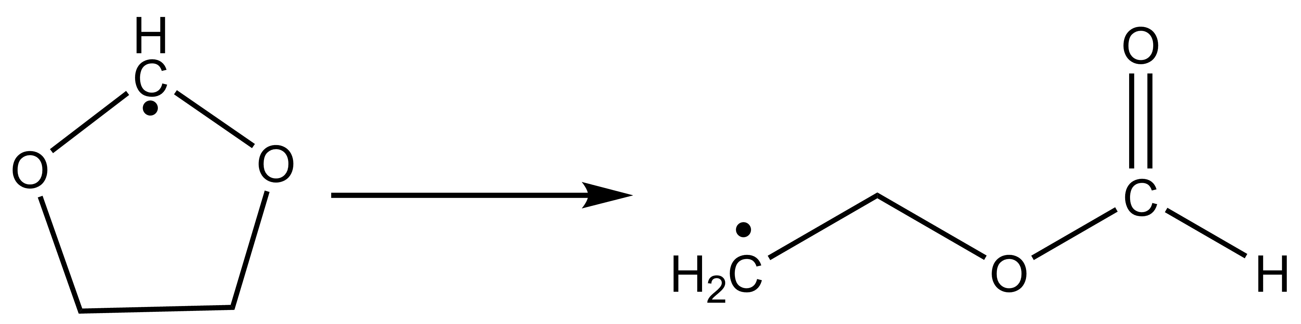
The high-level input for the IRC task is:

$irc
ircpts # Maximum number of steps for the reaction path
  50
ircdir # Direction of the reaction path
  0
ircalpha # Step size parameter for the reaction path
  0.05
$end
# The following parameters are the same as when calculating the TS structure
$compass
Title
  Irc4bdf
Geometry
C    -0.81981975    1.01964884    0.22750818
C     0.62889615    1.02275098   -0.13495924
O     1.14639042   -0.35161068    0.02899058
C     0.09835734   -1.20263633    0.05869588
O    -1.03508512   -0.71305587   -0.26218679
H -1.52425628 1.52979576 -0.43070061
H -1.07734340 1.04483316 1.29117725
H 0.79223623 1.32207879 -1.18212528
H 1.25263913 1.63815017 0.52777758
H 0.22167944 -2.05610649 0.75197182
End geometry
Basis
  CC-PVDZ
$end

$xuanyuan
$end

$scf
door
guess
readmo
dft
  GB3LYP
charge
  0
spinmulti
  2
mpec+cosx
Molden
$end

$resp
Geom
$end

Calculation Result Analysis After running the IRC task, BDF generates an additional 3c2o5h.irc file and a 3c2o5h.trj file.

The 3c2o5h.irc file retains the information of each step of the calculation; The 3c2o5h.trj’ file retains the trace file for each step.

where “3c2o5h.irc” will first give some basic user setup information,

  IRC wrapper for BDF - version 2023A

Using BDF from: $BDFHOME/sbin/bdfdrv.py

Parameters for this run:
  Algorithm:       1
  N. Points: 50
 Grad. Tol.:  0.0001
    Hessian: c3o2h5.hess
       Mode:       0
  Direction:       1
      Alpha: 0.0500
      Delta:  0.0500
Damp Factor:  0.0500
Damp Update: 0
Max. Pl.: 0.0100
      Guess: C3O2H5. TS.scforb

This will be followed by the calculation of the energy of each frame of the structure and the RMS Grad.

 ------------------------------------------------------------------------
Pt.                Energy RMS Grad.       Damp
 -------------------------------------------------------------------------
 @ 1-267.675550488 0.01427 5.00e-02
 @ 2 -267.679192880 0.00232 5.00e-02
 @ 3 -267.681201395 0.01348 5.00e-02
 @ 4-267.690625817 0.01357 5.00e-02
 @ 5 -267.696989174 0.01006 5.00e-02
 @ 6 -267.699945911 0.00574 5.00e-02
 @ 7 -267.701148839 0.00394 5.00e-02
 @ 8 -267.701644838 0.00262 5.00e-02
 @ 9 -267.701959150 0.00243 5.00e-02
 @ 10 -267.702145221 0.00170 5.00e-02
 @ 11 -267.702350215 0.00189 5.00e-02
 @ 12 -267.702476410 0.00117 5.00e-02
 @ 13 -267.702602274 0.00145 5.00e-02
 @ 14 -267.702713773 0.00096 5.00e-02
 @ 15 -267.702843816 0.00133 5.00e-02
 @ 16 -267.702921941 0.00113 5.00e-02
 @ 17 -267.702997038 0.00077 5.00e-02

Finally, if it converges normally, it will appear

----------------------------------------------
--             ENERGY INCREASED             --
--            GEOMETRY  MIGHT BE            --
--          VERY CLOSE TO A MINIMUM         --
--                                          --
--        IRC CALCULATION TERMINATED!       --
----------------------------------------------

In addition, “3c2o5h.trj” is to output the trajectory of each step in the form of the following,

10
IRC for BDF-irc-f point 1 E=  -267.6755505
C -0.774450  1.005021  0.227507
C  0.623378  1.023651 -0.134433
O  1.142071 -0.346726  0.029851
C  0.099686 -1.204880  0.058039
O -1.040129 -0.707532 -0.261197
H -1.538885 1.536311 -0.439412
H -1.084614 1.045208 1.295915
H 0.789098 1.321574 -1.178911
H 1.246292 1.636770 0.526219
H 0.221239 -2.055548 0.752570
10
IRC for BDF-irc-f point 2 E=  -267.6791929
C -0.806848  1.013333  0.225962
C  0.635583  1.022502 -0.136684
O  1.144366 -0.348838  0.029978
C  0.099054 -1.205298  0.056237
O -1.037689 -0.705204 -0.259469
H -1.515348 1.520972 -0.422025
H -1.076532 1.043033 1.285840
H 0.789437 1.322192 -1.180942
H 1.248393 1.638410 0.527357
H 0.220724 -2.055404 0.753891

Hint

To use the IRC module, the user needs to install numpy;
Users can input the obtained coordinate file into Device Studio to view the change of the trajectory, and this function will be updated on the DS platform.

The CI-NEB method was used to calculate the lowest energy path and optimize the transition state

With the original Pulled Rubber Band (Nudged Elastic Band; NEB) method, the CI-NEB method adds the image point climbing (Climbing Image; CI) processing steps, so that not only can we get a more accurate minimum energy (reaction) pathway, but also a transition state structure :cite:’neb2000’.

Again, take the example of HCN isomerization reaction in the previous section, and see the previous Dimer method for consideration. The CI-NEB calculation requires the provision of coordinates for two endpoints, where the initial structure of the first endpoint (here the reactant HCN) is provided in the Compass module, with a little perturbation added due to the linear structure being difficult to handle. The second endpoint is a curved structure (CI-NEB-optimized to become an HNC isomer), which is provided in the ‘’Geometry2’’ … ‘’End Geometry2’’ input block. The atomic order of the two sets of coordinates must be consistent. The input files are as follows:

$compass
basis-block
 def2-SVP
end basis
geometry
 C    0.0200000   0.0000000   0.0000000
 N 0.00000000 -1.1400000 0.0000000
 H 0.0000000 1.0500000 0.0000000
end geometry
nosymm
$end

$bdfopt
solver
 0
iopt
 3
neb-block
 crude
 nebmode
   0
 nimage
   3
end neb
geometry2
 C    0.0000000   0.0000000   0.0000000
 N -1.1500000 0.2300000 0.0000000
 H -1.6100000 1.1100000 0.0000000
end geometry2
$end

$xuanyuan
$end

$scf
rks
dft
 b3lyp
$end

$resp
 Geom
$end

Because the CI-NEB method has more intermediate image points, the slower the calculation and increases the probability that the structure will not converge, so it is not recommended to use too many intermediate image points, and it is recommended to use between 3 and 7. If you are only concerned with transition states, you can also try to use fewer intermediate image points, such as 1, but this is not feasible for this example, because the reactants and products are linear structures, while the intermediate image points are curved structures, As a result, the gradient vector overlap of the two is too small, which affects the structural convergence. In this example, 3 intermediate image points are used, defined by ‘’’Nimage’’’, and ‘’Crude’’ is used to reduce the convergence accuracy, while minimizing the energy of reactants and products (‘’Nebmode’’ = 0; fixed by default).

In addition to the 3 intermediate pixels specified by Nimage, there are 3 other pixels that must be counted, so the total number of pixels is 6. Among them, 1 and 5 image points correspond to two endpoints (i.e., reactants and products), and 2, 3, and 4 are intermediate image points on the reaction path. When these 5 image points are optimized to a certain extent, image point 6 is created for the climb step, which is eventually optimized to the transition state.

After 31 steps of structural optimization, the CI-NEB method found the lowest energy path:

Testing convergence of NEB climbing image in cycle   31
    Energy  7.1900E-07 Target: 4.0000E-05 converged?  yes
  Max step  1.1193E-03 Target: 5.3333E-03 converged?  yes component     8
  RMS step  6.5514E-04 Target: 3.5556E-03 converged?  yes
  Max grad  7.4900E-05 Target: 1.3333E-03 converged?  yes component     5
  RMS grad  3.6435E-05 Target: 8.8889E-04 converged?  yes
Convergence reached

Scroll forward to see the energy summary report of each image point (including reactants, products, and transition states):

NEB Report
             Energy       F_tang    F_perp     Dist     Angle 1-3 Ang 1-2 Sum
Img    1    -93.3003651   0.00000   0.00000   1.17248    0.00    0.00   63.25   frozen
Img    2    -93.2804319   0.00160   0.00059   1.01235   63.25   86.25   94.29   frozen
Img    3    -93.2270244  -0.00167   0.00049   1.17963   31.04   77.08   80.27   frozen
Img    4    -93.2512597  -0.00248   0.00075   1.42718   49.23    0.00   49.23   frozen
Img    5    -93.2785849   0.00000   0.00000   0.00000    0.00    0.00    0.00   frozen
Cimg   3    -93.2241949   0.00010   0.00007   0.21264    0.00    0.00    0.00

In the table above, the Energy column gives the energy of each image point in the reaction path, where the last Cimg represents the climbing image point, which is the transition state, And the closest image point to it (in this case, image point 3) is marked. The F_tang and F_perp columns give the forces on each image point in the direction of the parallel and perpendicular paths, which should be close to zero in principle. The Dist, Angle, 1-3 Ang, and 1-2 Sum columns give the characteristics of the path, which are the distance from the current image point to the next image point (you can see that the image point of NEB is no longer equally spaced after optimization), The angle of the current image point to the previous image point, the angle of the next image point to the previous image point, and the sum of the angles of the current image point and the next image point. By adding up the data in the Dist column as the horizontal axis and the energy as the vertical axis, you can plot the energy plot of the NEB reaction coordinates (these data can be found in a separate file nebinfo).

The total energy of the transition state given in this line is -93.2241949 Hartree (the final converged energy printed by DL-FIND is also this energy), which is very close to the total energy of the transition state of -93.22419648 Hartree optimized by the previous Dimer method.

The Cartesian coordinates of the transition state can be found before the energy data (atomic units) and are also printed at the end of the text file neb_0006.xyz saved by CI-NEB (since the transition state is the sixth image point in this case) in angstroms. The Cartesian coordinates of the remaining 5 image points are saved in the nebpath.xyz of a text file (unit: angstroms). If necessary, the transition state structure can also be optimized more rigorously using the method described above, which is more efficient than using the strict convergence criterion directly in the CI-NEB calculation.

The energy of the optimized image point at each step is extracted, and the NEB trajectory diagram is drawn as follows. As a demonstration, the horizontal coordinates are taken from the last step, but there are actually some variations in the horizontal coordinates for each step.

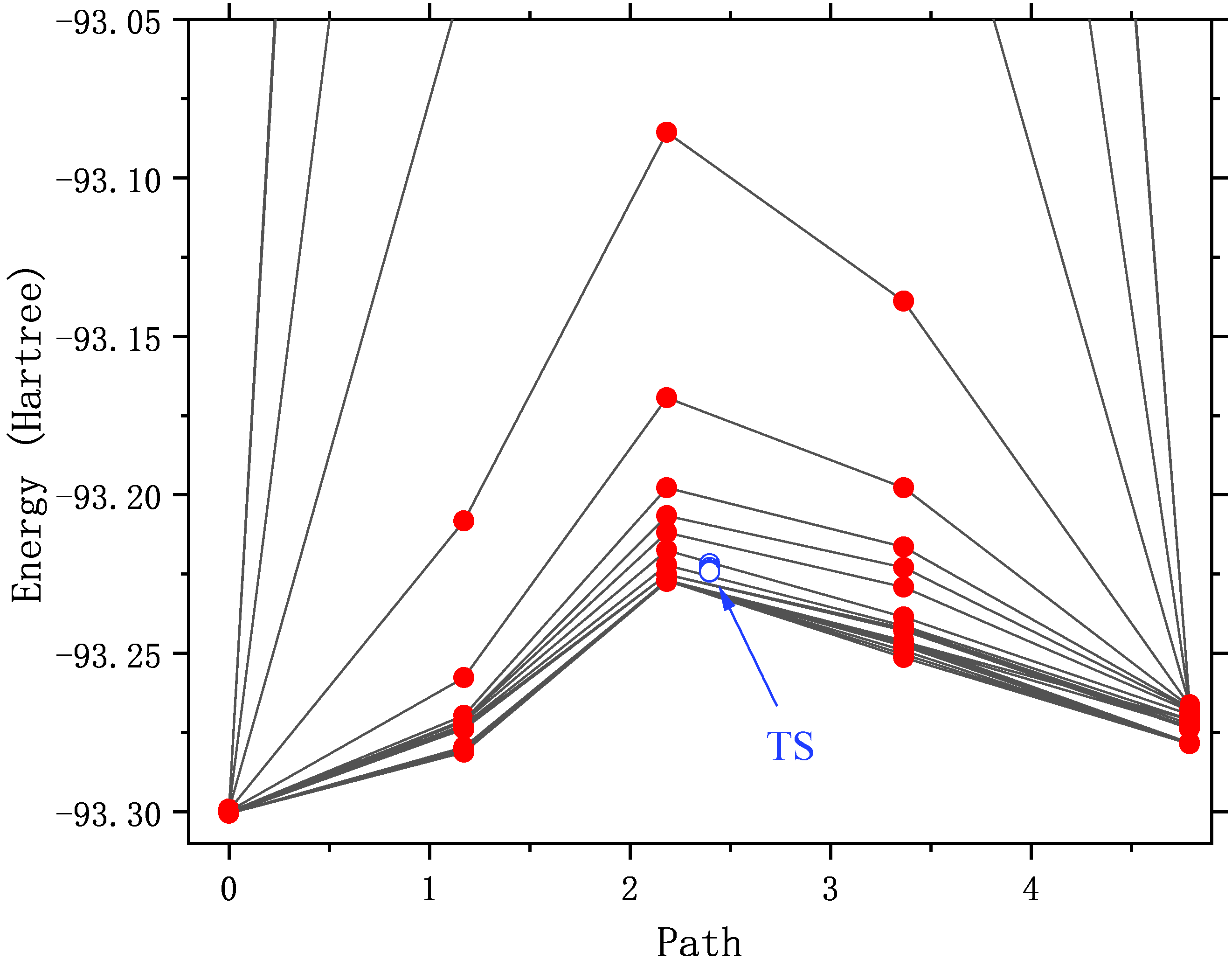
It can be seen that with the optimization, the energy of the path gradually decreases until it converges. As you may have noticed, the energy of pixels 2 to 4 is very high (out of the display range) in the first few rounds of structural optimization. Illustrates that the initial structure of these points is not quite reasonable. For example, in the initial structure of the No. 3 image spot, the C-N bond is only 0.5 angstrom long! An unreasonable structure will not only hinder the structural convergence, but also destroy the SCF convergence. Or converge to an excited state that we don’t want.

CI-NEB calculations often do not converge. There are the following ways to deal with it:

Extract the structure of the image point with the highest energy or the structure of the climbing image point, and use the transition state optimization method described above to calculate it instead.
Extract the structures of the two image points with the highest energy (e.g., 3 and 4 in this example) as the initial structure, and redo the CI-NEB optimization, but at this time, the “Nebmode” should be changed to 1 or 2, because they are no longer reactants, products, or intermediates, and there is no point in doing energy minimization.
Take the two endpoint structures of the last step of structure optimization, and some or all of the intermediate image point structures (from the data file nebpath.xyz) as the initial structure, and redo the CI-NEB optimization. The input files are as follows. In this example, the structure of both endpoints is already close to convergence (both F_tang and F_perp are very small), and in order to increase the computation speed, the structure remains frozen (Nebmode’ = 2).

$compass
basis-block
 def2-SVP
end basis
geometry
# geom of image 1 (endpoint 1)
C       0.0094403     -0.0045178      0.0000000
N 0.0051489 -1.1595576 0.0000000
H 0.0054108 1.0740754 0.0000000
end geometry
norotate
$end

$bdfopt
solver
 0
iopt
 3
Trust
 0.02
neb-block
 crude
 nebmode
   2
 nimage
   3
end neb
nframe
  4
geometry2
# geom of image 2
C       0.2822075     -0.0905533      0.0000000
N -0.4636856 -0.9729686 0.0000000
H 0.2014782 0.9735219 0.0000000
# geom of image 3
C       0.5703159     -0.2134900      0.0000000
N -0.5233808 -0.6609221 0.0000000
H -0.0269352 0.7844121 0.0000000
# geom of image 4
C       0.7857794     -0.5068651      0.0000000
N -0.3940425 -0.3160241 0.0000000
H -0.3717369 0.7328892 0.0000000
# geom of image 5 (endpoint 2)
C       0.5798873     -0.9890158      0.0000000
N -0.0251869 0.0162146 0.0000000
H -0.5347005 0.8828012 0.0000000
end geometry2
$end

$xuanyuan
$end

$scf
rks
dft
 b3lyp
$end

$resp
 Geom
$end

A little trick is used here: in the automatically generated intermediate image point coordinates, the z-direction coordinates may be non-zero, and in the case of triatomic molecules, the keyword “Norotate” will conflict with the symmetry program. Therefore, the symmetry had to be turned off with “Nosymm” in front. Now that we have qualitatively correct image point coordinates, we can zero out the small values of these coordinates in the z direction. Then change “Nosymm” to “Norotate” so that you can take advantage of the Cs symmetry to speed up the calculation.

Redraw the NEB trajectory as shown in the figure below. Since the intermediate image point uses a good initial structure, the energy in the first few steps of optimization is reasonable.

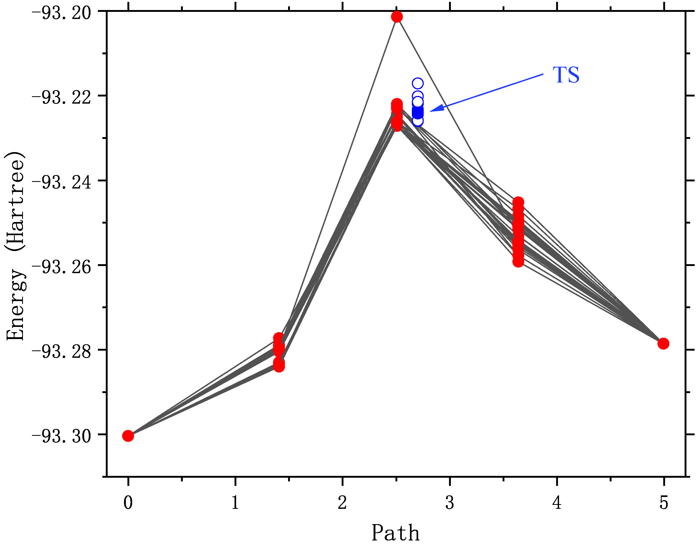
Structural optimization of spin hybrid states: ZnS molecules

The ground state of the diatomic molecule ZnS is closed-shell :math:’X^1Sigma^+’ with a bond length of 2.05 angstroms, and the first excited state above 11 kcal/mol is math:’^3Pi’, Crossover with the ground state near 2.4 angstrom :cite:’PSS2007’. The :math:’^3Pi_{0+}’ component of the excited state interacts with the ground state, The bond length that may affect the ground state.

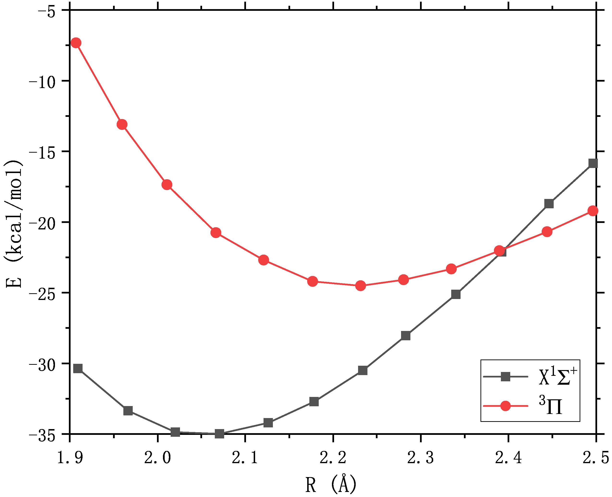
If accuracy is not required, the spin-orbit model Hamiltonian proposed by Truhlar et al. can be used to simulate the spin-orbit coupling between two spin states. Consider the effect of :math:’^3Pi_{0+}’ on the ground state. The input files are as follows. Among them, the ground state is completed with RKS, and the lowest triple excited state is completed with UKS. There are a few things to note in the input file:

Note

The option for two-state hybrid computing is “2SoC” (similar to “3SoC”, “4SoC”, etc.). In general, these two spin states need to have different spin multiplicities, unless theoretical calculations prove that there is also a strong SOC interaction between two states with the same spin (e.g., the :math:’^2D_u’ and :math:’^2P_u’ of nitrogen atoms).
The empirical value of the spin-orbit coupling constant set here is 400 :math:’rm cm^{-1}’ which happens to be the default value of the program, so it can be omitted and not written.
Specify the BDF’s built-in optimizer with ‘’solver’’ = 1. You can also use the DL-Find optimizer, but it is generally slower.
The energies and gradients of the two spin states should be saved to the $BDFTASK.egrad.1 and $BDFTASK.egrad.2 files, respectively. As for which state is specified as No. 1 or No. 2, it is entirely up to the user to decide and does not affect the final result.
In the process of BDF structure optimization, the SCF orbital saved in the previous step is used as the initial guess of the current SCF step by default to obtain the fastest SCF convergence. Since the two SCF calculations use different SCF pre-guess orbitals, They need to be backed up as $BDFTASK.scforb.1 and $BDFTASK.scforb.2, respectively. However, when overwriting $BDFTASK.scforb with them for the first time, since the SCF calculation has not yet been performed,

If these two files do not exist, the replication error will occur, and the BDF will stop the calculation when it finds out. In order to block out the error copying message, you need to add 2>/dev/null to the end of the copy command.
The lowest triple excited state can also be calculated by spin flipping using TDDFT, which requires adding some additional keywords to the $tddft’ and $resp’ (see the TDDFT section <TDDFTopt>’). However, TDDFT does not describe the charge transfer state well (this is the case with ZnS) and is not used here.

$COMPASS
Title
 two-state calculation of ZnS
Basis
 lanl2dz
Geometry
 Zn 0.0 0.0 0.0
 S   0.0  0.0  2.05
END geometry
$END

$bdfopt
solver
 1
multistate
 2soc  400
$end

$xuanyuan
$end

%cp $BDF_WORKDIR/$BDFTASK.scforb.1   $BDF_WORKDIR/$BDFTASK.scforb    2>/dev/null || :

$SCF
rks
dft
 pbe0
charge
 0
spinmulti
 1
$END

%cp $BDF_WORKDIR/$BDFTASK.scforb     $BDF_WORKDIR/$BDFTASK.scforb.1

$resp
Geom
$end

%cp $BDF_WORKDIR/$BDFTASK.egrad1     $BDF_WORKDIR/$BDFTASK.egrad.1

%cp $BDF_WORKDIR/$BDFTASK.scforb.2   $BDF_WORKDIR/$BDFTASK.scforb    2>/dev/null || :

$SCF
door
dft
 pbe0
charge
 0
spinmulti
 3
$END

%cp $BDF_WORKDIR/$BDFTASK.scforb     $BDF_WORKDIR/$BDFTASK.scforb.2

$resp
Geom
$end

%cp $BDF_WORKDIR/$BDFTASK.egrad1     $BDF_WORKDIR/$BDFTASK.egrad.2

After the calculation, the optimized spin mixed ground-state bond length is 2.1485 angstroms, which is slightly longer than the bond length of the pure single-weight ground state of 2.1480 angstroms (this value is much larger than the high-precision theoretical value of 2.05 angstroms, because the basis group used in this example is too small). Description :math:’^3Pi_{0+}’ elongates the bond length of the ground state by spin-orbit coupling. The output of the last optimized step shows that :math:’^3Pi_{0+}’ accounts for 0.2% of the spin mixed ground state.

Multi-state calculation
-----------------------

Mixed-spin states by 2 scalar states.

Chi =  400.0 cm^-1 is used to constuct the SO model Hamiltonian.

/tmp/zouwl/BDF-1/test.egrad.1
  E=           -75.49718339
/tmp/zouwl/BDF-1/test.egrad.2
  E=           -75.46038704

Energies and weights of mixed-spin states:
------------------------------------------------------------------
 No.            E(mix)            Weights
------------------------------------------------------------------
  1           -75.49727344        99.8%     0.2%
  2           -75.46029699         0.2%    99.8%
------------------------------------------------------------------

In addition to optimizing the structure of the spin mixed ground state, it is also possible to calculate its vibrational frequency, for which the Hessian of the two spin states needs to be saved to the $BDFTASK.hess.1 and $BDFTASK.hess.2 files, respectively.

If you want to calculate the frequency only on the optimized structure, similar to the input above for the optimized structure, just change “solver” = 1 to “hess” = “only”, and change the backup gradient file “$BDFTASK.egrad1” to the backup Hessian file “$BDFTASK.hess”.
When doing structural optimization + frequency calculation, the input needs to be modified additionally. This is because there is no Hessian file in the optimization process, and there is no gradient file in the frequency calculation process, so you have to use ‘’2>/dev/null || :’’ Mask out messages that are duplicated incorrectly. The input files that work properly are as follows:

$COMPASS
Title
 two-state calculation of ZnS
Basis
 lanl2dz
Geometry
 Zn 0.0 0.0 0.0
 S   0.0  0.0  2.05
END geometry
$END

$bdfopt
solver
 1
multistate
 2soc  400
hess
 final
$end

$xuanyuan
$end

%cp $BDF_WORKDIR/$BDFTASK.scforb.1   $BDF_WORKDIR/$BDFTASK.scforb    2>/dev/null || :
$SCF
rks
dft
 pbe0
charge
 0
spinmulti
 1
$END
%cp $BDF_WORKDIR/$BDFTASK.scforb     $BDF_WORKDIR/$BDFTASK.scforb.1

$resp
Geom
$end

%cp $BDF_WORKDIR/$BDFTASK.egrad1     $BDF_WORKDIR/$BDFTASK.egrad.1   2>/dev/null || :
%cp $BDF_WORKDIR/$BDFTASK.hess $BDF_WORKDIR/$BDFTASK.hess.1 2>/dev/null || :

%cp $BDF_WORKDIR/$BDFTASK.scforb.2   $BDF_WORKDIR/$BDFTASK.scforb    2>/dev/null || :
$SCF
door
dft
 pbe0
charge
 0
spinmulti
 3
$END
%cp $BDF_WORKDIR/$BDFTASK.scforb     $BDF_WORKDIR/$BDFTASK.scforb.2

$resp
Geom
$end

%cp $BDF_WORKDIR/$BDFTASK.egrad1     $BDF_WORKDIR/$BDFTASK.egrad.2   2>/dev/null || :
%cp $BDF_WORKDIR/$BDFTASK.hess $BDF_WORKDIR/$BDFTASK.hess.2 2>/dev/null || :

The main purpose of the polymorphic mixing model is to study polymorphic reactions, optimize the reactants, intermediates, products, transition states of the spin mixed state, and reaction pathways. It provides more information than MECP optimization (e.g., if MECP results in a new transition state, a polymorphic hybrid model can estimate the vibrational frequencies and thermochemical quantities in the vicinity of MECP). When the atoms are not too heavy (before 5d), the polymorphic mixed model has many advantages over the two- or four-component relativistic approach, which strictly considers the rotation-orbit coupling.

Restrictive structure optimization

BDF also supports restricting the value of one or more internal coordinates in structural optimization by adding the constrain keyword to the BDFOPT module. The first line after the constrain keyword is an integer (hereinafter referred to as N), representing the total number of restrictions; Lines 2 to N+1 define each limit. For example, the following input indicates that the distance between the 2nd and 5th atoms is limited for structural optimization (there is not necessarily a chemical bond between these two atoms):

$bdfopt
solver
 1
constrain
 1
 2 5
$end

The following inputs indicate that the distance between the 1st and 2nd atoms is limited to the 2nd atom during the structural optimization, while also limiting the bond angle formed by the 2nd, 5th, and 10th atoms (again, there is no requirement for the 2nd and 5th atoms, or the chemical bonds between the 5th and 10th atoms):

$bdfopt
solver
 1
constrain
 2
 1 2
 2 5 10
$end

The following inputs represent the dihedral angle between the 5th, 10th, 15th, and 20th atoms and the dihedral angle between the 10th, 15th, 20th, and 25th atoms at the time of structural optimization:

$bdfopt
solver
 1
constrain
 2
 5 10 15 20
 10 15 20 25
$end

Note

Even if the numerator coordinates are entered as Cartesian coordinates instead of internal coordinates, the BDF can still be restrictively optimized for the internal coordinates.

When it is necessary to freeze multiple atoms at the same time (for example, to study a surface catalytic reaction using a cluster model, and want to freeze a subset of catalyst atoms), although it is still possible to exhaust all the bond lengths, bond angles, and dihedral angles between these atoms and freeze them one by one, it is troublesome and error-prone when the number of atoms that need to be frozen is large. Therefore, BDF also supports the ability to freeze the Cartesian coordinates of atoms by using the frozen keyword. For example:

$bdfopt
...
frozen
 3 # number of atoms to be frozen
 2 -1
 5 -1
 10 -1
$end

Indicates the freezing of atoms 2, 5, and 10. When using the DL-Find optimizer (i.e., solver=0), -1 can also be replaced with a different number to freeze only one or both of the x, y, and z coordinates of that atom:

  0: free (default)
 -1: frozen
 -2: x frozen only
 -3: and Frozen Only
 -4: With Frozen Only
-23: x and y frozen
-24: X and Z Frozen
-34: Y and Z Frozen

For example

$bdfopt
...
frozen
 4 # number of atoms to be frozen
 3 -1
 4 -1
 5 -1
 6 -4
$end

That is, the Cartesian coordinates of atoms 3~5 and the z coordinates of atom 6 are frozen, but atom 6 can still move freely in the x and y directions.

Note

The program freezes the relative Cartesian coordinates between the atoms specified by the user, and the absolute Cartesian coordinates of the atoms may still change due to the change of the standard orientation of the molecule;
The same calculation can freeze both any number of Cartesian coordinates and any number of inner coordinates.

For the calculation of frozen internal coordinates, the program also supports freezing the inner coordinates to a value that is different from the initial structure. For example, in the following input file, the structure of ethylene oxide is optimized at the M06-2X/6-31+G(d,p)/SMD(water) level, but the length of one of the C-O bonds is limited to 2.0 angstroms:

$compass
Geometry
 C                  0.00000000    0.70678098   -0.40492819
 C                  0.00000000   -0.70678098   -0.40492819
 O                  0.00000000    0.00000000    0.95133348
 H 0.86041653 1.24388179 -0.74567167
 H -0.86041653 1.24388179 -0.74567167
 H 0.86041653 -1.24388179 -0.74567167
 H -0.86041653 -1.24388179 -0.74567167
End Geometry
Basis
 6-31+G(d,p)
MPEC+COSX
$end

$bdfopt
Solver
  1
constraint
 1 # number of constraints
 2 3 = 2.0 # constrain the distance of atom 2 and atom 3 at 2.0 Angstrom
$end

$xuanyuan
$end

$scf
RKS
dft
 M062X
Solmodel
 SMD
solvent
 water
$end

$resp
Geom
$end

In the initial structure, both C-O bonds had a bond length of 1.53 angstroms, but after optimizing convergence, it can be found that the frozen C-O bond has a bond length of exactly 2.00 angstroms (instead of 1.53 angstroms), and the other C-O bond length without freezing is optimized to 1.43 angstroms:

|******************************************************************************|
       Redundant internal coordinates on Angstrom/Degree

  Name         Definition         Value     Constraint
  R1 1 2 1.4907 No
  R2 1 3 1.4332 No
  R3 1 4 1.0917 No
  R4 1 5 1.0917 No
  R5          2   3               2.0000    Yes
  R6 2 6 1.0845 No
  R7 2 7 1.0845 No
  A1 2 1 3 86.29 No
...

In the same calculation, only a part of the coordinates can be assigned, and the rest of the coordinates automatically inherit the values in the initial structure. For example, the following input is valid, indicating that the Cartesian coordinates of atoms 1, 2, and 5 are frozen, and the bond angles of atoms 5-6-8 are frozen, and the dihedral angles of atoms 11-12-13-14 are frozen. For example, if the dihedral angle of atoms 11-12-13-14 in the initial structure is 120 degrees, the dihedral angle of atoms 11-12-13-14 is always 120 degrees in the subsequent structural optimization:

$bdfopt
...
solver
 1
frozen
 3
 1 -1
 2 -1
 5 -1
constrain
 2
 5 6 8 = 60.
 11 12 13 14
$end

Note

The program only supports setting the values of the frozen key length, key angle, and dihedral angle, but does not support setting the Cartesian coordinate value of the frozen atom when freezing the Cartesian coordinates.

When you freeze multiple internal coordinates at the same time and assign values, you need to confirm that the frozen internal coordinates are self-consistent with each other. As an example of internal coordinate inconsistency, consider the following input:

$bdfopt
Solver
  1
constraint
 3
 1 2 = 1.0
 1 3 = 2.0
 2 3 = 4.0
$end

Obviously, these three bond length constraints cannot be met at the same time, because it is not possible to form a triangle from three bonds with bond lengths of 1 angstrom, 2 angstroms, and 4 angstroms. When the program finds that it cannot meet all three conditions at the same time, it prints a warning message:

  q2c_coord_calc: warning: the   1-th constraint cannot be enforced, error =  0.204E+00
Check if the input constraints are mutually contradictory, or numerically ill-posed!
  q2c_coord_calc: warning: the   2-th constraint cannot be enforced, error =  0.200E+00
Check if the input constraints are mutually contradictory, or numerically ill-posed!
  q2c_coord_calc: warning: the   3-th constraint cannot be enforced, error = -0.149E+01
Check if the input constraints are mutually contradictory, or numerically ill-posed!

Finally, because the optimizer could not be solved after restarting the optimizer several times, the program returned an error and exited.

Note

In the above example, it is mathematically impossible to satisfy all the constraints of the inner coordinates at the same time. Sometimes, although it is mathematically possible to satisfy all the constraints at the same time, but the initial structure is too far away from the structure that satisfies the constraints, the program may still not find a structure that satisfies all the constraints at the same time, and print a warning or exit with an error.

Optimization of excited state structure

In addition to optimizing the ground state structure, the BDF program can also optimize the excited state structure, please refer to the relevant section of TDDFT <TDDFTopt> for details, which will not be repeated here.

QM/MM structure optimization

BDF can also use the QM/MM combination method for structural optimization, but unlike pure QM structural optimization, QM/MM structural optimization cannot be completed using the BDFOPT module, but must use the built-in structural optimization function of the pDynamo program. For details, please refer to the QM/MM section <QMMMopt> and will not be repeated here.

Automatically eliminate virtual frequencies

Whether it is to optimize the structure of the minimum point or the transition state, the number of virtual frequencies of the optimized convergence structure is often not consistent with the expectation, which can be divided into three categories: (1) the structure of the optimized minimum point convergence has virtual frequencies; (2) There is more than one imaginary frequency of the structure of the optimized transition state convergence; (3) The structure of the convergence of the optimized transition state has no imaginary frequency. For (1) and (2), BDF can automatically eliminate excess virtual frequencies, for which the keyword ‘’rmimag’’ (or ‘’removeimag’’) needs to be added to the input of the BDFOPT module; This keyword also has a certain effect on the case (3), that is, when there is no virtual frequency in the optimization transition state result, it is possible to find a structure with an imaginary frequency nearby, but the success rate is low. For example, the following input means that the minimum point structure is optimized, and then a frequency calculation is made, and the calculation is terminated if there is no imaginary frequency; If there is a virtual frequency, the molecular structure will be automatically perturbed along the direction of the vibration mode corresponding to the virtual frequency with the largest absolute value, and then continue to optimize, and then do a frequency calculation to verify whether the virtual frequency has been eliminated after optimization and convergence, and so on until all the virtual frequencies are completely eliminated, or the frequency has been calculated 10 times and all the virtual frequencies are still not eliminated:

$bdfopt
solver
1
rmimag
$end

The following input works similarly to the above input, except that a full frequency analysis and thermochemical analysis are performed on the last calculated Hessian:

$bdfopt
solver
1
rmimag
hess
 final
$end

The following input indicates that the transition state structure is optimized (a frequency calculation is done before the optimization begins, to provide the initial Hessian for the structure optimization), followed by a frequency calculation, and the calculation is completed if there is exactly one imaginary frequency. If the number of virtual frequencies is greater than 1, the molecular structure will be automatically perturbed along the direction of the second largest virtual frequency in absolute value, and then continue to optimize, and then do a frequency calculation to verify whether the excess virtual frequencies have been eliminated after optimization convergence, and so on until the number of virtual frequencies is equal to 1. If the number of virtual frequencies is equal to 0, it automatically tries to find a structure with a virtual frequency number equal to 1 nearby, and after optimizing the convergence, the frequency is also recalculated to verify the virtual frequency number, and so on until the virtual frequency number is equal to 1:

$bdfopt
solver
1
rmimag
hess
 init # calculate initial Hessian. If a thermochemistry analysis on the final Hessian is desired, change “init” to “init+final”
iopt
 10 # transition state optimization
$end

The following is a complete example of an optimized equilibrium structure for :math:’ce{ClF3}’ at HFLYP/6-31G(d) level:

$compass
title
 ClF3
basis
 6-31G(d)
geometry
Cl 0.0000000 0.0000000 0.0000000
F -2.966870 0.000000 0.000000
F 1.483435 2.569385 0.000000
F 1.483435 -2.569385 0.000000
end geometry
unit
 bohr
nosymm
$end

$bdfopt
solver
 1
rmimag
hess
 final
$end

$xuanyuan
$end

$scf
rks
dft
 HFLYP
$end

$resp
Geom
$end

The initial structure conforms to the :math:’rm D_{3h}’ symmetry, but because the structure of the expected optimal convergence may have virtual frequencies, it is specified in the ‘’compass’ module with the ‘’’nosymm’’ keyword to be calculated under the :math:’rm C_{1}’ group. The program first converges to the minimum point under the :math:’rm D_{3h}’ point cluster:

|******************************************************************************|
       Redundant internal coordinates on Angstrom/Degree

  Name         Definition         Value     Constraint
  R1 1 2 1.6666 No
  R2 1 3 1.6667 No
  R3 1 4 1.6667 No
  A1 2 1 3 119.99 No
  A2 2 1 4 119.99 No
  A3 3 1 4 120.02 No
  D1 4 1 3 2 179.97 No
  D2 2 1 4 3 179.97 No
  D3 3 1 4 2 -179.97 No

|******************************************************************************|

Then restart the Structure Optimizer:

--- Restarting optimizer ... (10 attempt(s) remaining) ---

Next, the program performs a numerical Hessian calculation and finds that the structure has two imaginary frequencies:

Warning: the number of imaginary frequencies,  2, is different from the desired number,  0!

Therefore, the program perturbates the structure and continues to optimize it in order to eliminate the virtual frequency. Because the angle of an F-Cl-F bond is close to 180°, the redundant internal coordinates need to be reconstructed, resulting in the restart of the structure optimizer. Finally, the convergence yields a T-shaped structure belonging to the :math:’rm C_{2v}’ point group:

|******************************************************************************|
       Redundant internal coordinates on Angstrom/Degree

  Name         Definition         Value     Constraint
  R1 1 2 1.5587 No
  R2 1 3 1.6470 No
  R3 1 4 1.6470 No
  R4 2 4 2.1859 No
  A1 2 1 3 85.95 No
  A2 2 1 4 85.94 No

|******************************************************************************|

Finally, the structure optimizer is restarted for the third time, and the Hessian calculation confirms that the structure has no virtual frequencies, that is, the first two imaginary frequencies have been eliminated. At this point, the entire computation declares convergence:

***************************************  Properties of Normal Modes  ***************************************

Results of vibrations:
Normal frequencies (cm^-1), reduced masses (AMU), force constants (mDyn/A)

                                                  1                                 2                                 3
         Irreps                                  A"                                A'                                A'
    Frequencies                            385.8687                          414.4702                          519.9076
 Reduced masses                             24.3196                           21.5030                           19.4352
Force constants                              2.1335                            2.1764                            3.0952

Note

The program does not guarantee that all excess virtual frequencies will be eliminated in all cases, and even if the program ends normally, the number of virtual frequencies may still be wrong. Therefore, even if the “rmimag” keyword is added, the user still needs to check the number of virtual frequency after the optimization is completed. If the number of virtual frequencies is still not equal to the expected value (i.e., for minimum point optimization, there are still virtual frequencies; Or for transition-state optimization, where there are no virtual frequencies or the number of virtual frequencies is greater than one), you need to manually handle the virtual frequency problem <removeimagfreq>’ subsection :ref:.
If the molecule has point group symmetry, but no ‘’nosymm’’ is specified in the calculation, it may not be possible to completely eliminate all the virtual frequencies, and may even lead to non-convergence of structural optimization. For example, in the above example, if nosymm is not specified, and the calculation is performed under the actual point group of the molecule ( :math:’rm D_{3h}’ ), the optimization will not converge because eliminating the two imaginary frequencies will break the :math:’rm D_{3h}’ symmetry.
The structure obtained by restrictive optimization (regardless of whether it is restricted to Cartesian coordinates or internal coordinates) may (but not necessarily) have imaginary frequencies that cannot be eliminated. In this case, if the number of virtual frequencies is greater than expected, it does not necessarily mean that the current structure is unavailable. By observing the vibration patterns of the virtual frequencies, the user should determine for himself whether the virtual frequencies are caused by the constraints imposed during optimization, and then determine whether these virtual frequencies should be eliminated.

Optimization of conical crossings (CI) and lowest energy crossings (MECP).

To optimize CI and MECP, you need to call the DL-FIND external library :cite:’dlfind2009’, for which you need to add the following keywords to the input of the BDFOPT module

solver
 0

Correspondingly, the ‘’solver 1’’ in each of the above studies means that the BDF’s built-in structural optimization code is used instead of DL-FIND for optimization. In principle, DL-FIND can also be used to optimize minimum points and transition states, but the efficiency is generally not as good as that of BDF’s own code, so DL-FIND should only be called for tasks that are not supported by BDF’s built-in code, such as CI and MECP optimization.

The following is an example input for CI optimization, which calculates the conical intersection of the T1 and T2 states of ethylene:

#----------------------------------------------------------------------
# Gradient projection method for CI between T1 and T2 by TDDFT BHHLYP/6-31G
#

$COMPASS
Title
   C2H4 Molecule test run
Basis
   6-31G
Geometry
 C                  0.00107880   -0.00318153    1.43425054
 C                  0.00066030    0.00195132   -1.43437339
 H 0.05960990 -0.89114967 0.84012371
 H -0.05830329 0.95445870 0.96064844
 H 0.05950228 0.89180839 -0.84311032
 H -0.06267534 -0.95390169 -0.95768311
END geometry
nosymm
$END

$bdfopt
imulti # Optimize CI
 2
maxcycle           # Maximum number of optimization steps
 50
Tolgrad # Convergence criterion for root mean square gradient
 1.d-4
Tolstep # Convergence criterion for root mean square step size
 5.d-3
$end

$xuanyuan
$end

$SCF
RKS
charge
 0
spinmulti
 1
atomorb
DFT
 BHHLYP
$END

$tddft
imethod
 1
ISF
 1
Itda
 1
nroot
 5
idiag
 1
istore
 1
crit_e
 1.d-8
crit_vec
 1.d-6
lefteig
ialda
 4
$end

$resp
Geom
norder
 1
method
 2
iroot
 1
nfiles
 1
$end

$resp
Geom
norder
 1
method
 2
iroot
 2
nfiles
 1
$end

$resp
iprt
 1
QUAD
FNAC
double
norder
 1
method
 2
nfiles
 1
pairs
 1
 1 1 1 1 1 2
$end

Note that this task not only needs to calculate the gradient of T1 and T2 states, but also needs to calculate the non-adiabatic coupling vector between T1 and T2 states (completed by the last RESP module), and the relevant keywords can be found in :d oc:’tddft’, which will not be repeated here. In the input of the BDFOPT module, ‘’imulti 2’’’ stands for Optimized CI. Similar to normal structure optimization tasks, CI optimization outputs the gradient and step length convergence for each step, as well as the energy convergence. For example, the output of the last optimization step of the above study is:

Testing convergence  in cycle    6
    Energy  0.0000E+00 Target: 1.0000E-06 converged?  yes
  Max step  9.0855E-04 Target: 5.0000E-03 converged?  yes component     4
  RMS step  5.6602E-04 Target: 3.3333E-03 converged?  yes
  Max grad  5.5511E-05 Target: 1.0000E-04 converged?  yes component     1
  RMS grad  2.7645E-05 Target: 6.6667E-05 converged?  yes
Converged!
 converged

Similar to the above-mentioned optimization tasks, the convergent CI structure is stored in the .optgeom file with Bohr coordinates. Note that the value of the energy row is always displayed as 0, which does not mean that the energy of the system remains unchanged during CI optimization, but because the convergence of energy will not be used to determine whether the convergence is used in the optimization CI. For the same reason, the keyword “tolene” is not useful for CI optimization (and MECP optimization below).

Here’s an example input file for optimizing MECP:

#----------------------------------------------------------------------
# Gradient projection method for MECP between S0 and T1 by BHHLYP/6-31G
#

$COMPASS
Title
   C2H4 Molecule test run
Basis
   6-31G
Geometry
C            -0.00000141      0.00000353      0.72393424
C             0.00000417     -0.00000109     -0.72393515
H 0.73780975 -0.54421247 1.29907106
H -0.73778145 0.54421417 1.29907329
H 0.73777374 0.54421576 -1.29907129
H -0.73779427 -0.54423609 -1.29906321
END geometry
nosymm
$END

$bdfopt
Multi
 2
maxcycle
 50
tolgrad
 1.d-4
tolstep
 5.d-3
noncouple
$end

$xuanyuan
$end

$SCF
RKS
charge
 0
spinmulti
 1
atomorb
DFT
BHHLYP
$END

$resp
Geom
norder
 1
method
 1
$end

$SCF
DOOR
charge
 0
spinmulti
 3
atomorb
DFT
BHHLYP
$END

$resp
Geom
norder
 1
method
 1
$end

The keywords ‘’imulti 2’’ and ‘’noncouple’’ are specified for MECP optimization. Note that the MECP optimization task only needs to compute the gradient of the two states (in this case, the S0 state and the T1 state), and does not need to calculate the non-adiabatic coupling vector. The output of the MECP optimization task is similar to that of the CI optimization task, and will not be repeated here.

Geometry Optimization FAQs

False frequency issues

Geometry optimization not only requires the structure to converge (i.e., the gradient and step size meet the convergence limit requirements), but also requires that the number of imaginary frequencies of the obtained structure conforms to the expected value, that is, when the minimum value point structure is optimized, the number of imaginary frequencies is 0. When the transition state is optimized, the number of virtual frequencies is 1; If the number of imaginary frequencies is greater than 1, it is a higher-order saddle point. When the actual number of virtual frequencies calculated does not match the expected value, the structure needs to be adjusted and re-optimized. In general, the problem of too many virtual frequencies and a small number of low virtual frequencies can be solved by using the rmimag keyword <rmimag> in small quantities. When the rmimag keyword does not work, you should manually resolve the issue where the number of virtual frequencies does not meet your expectations as follows:

When the actual number of virtual frequencies calculated is less than the expected value, that is, the structure with the number of imaginary frequencies is 0 obtained by optimizing the transition state: at this time, it is generally explained that the qualitative error of the obtained transition state structure is required, and the initial guess structure needs to be re-prepared according to chemical knowledge.

When the actual number of calculated virtual frequencies is greater than the expected value, there are two possible situations: (1) The virtual frequency is caused by the numerical error of the calculation, and it is not real. In this case, it can be solved by increasing the grid point, decreasing the integration truncation threshold, and decreasing various convergence thresholds (such as SCF convergence threshold, structure optimization convergence threshold, etc.). (2) There is indeed a virtual frequency in the system. In this case, the normal mode corresponding to the virtual frequency should be checked from the output file, and the convergent structure should be perturbed along the direction of the normal mode, and then the structure after the disturbance should be used as the initial structure to re-optimize.

Note that it is not possible to determine whether an imaginary frequency is caused by a numerical error based on the frequency calculation results alone, but in general, the smaller the absolute value of the imaginary frequency, the more likely it is to be caused by a numerical error, and vice versa.

Structures obtained by restrictive optimization (regardless of whether they are constrained by Cartesian or internal coordinates) may (but are not necessarily) have virtual frequencies that cannot be eliminated. In this case, if the number of virtual frequencies is greater than expected, it does not necessarily mean that the current structure is unavailable. By observing the vibration patterns of the virtual frequencies, the user should determine for himself whether the virtual frequencies are caused by the constraints imposed during optimization, and then determine whether these virtual frequencies should be eliminated.

Symmetry issues

When the initial structure has the symmetry of the point group above the :math:’rm C_1’ group, the structure optimization may break the point group symmetry, for example, when optimizing the ammonia molecule, the initial structural symmetry of the planar structure is :math:’rm D_{3h}’, the structure optimization may obtain a tapered structure with symmetry of :math:’rm C_{3v}’. By default, BDF enforces the symmetry of the molecular point group, unless there is a first-order Jahn-Teller effect in the system. If the user wants BDF to break the symmetry of the molecule, one of the following methods can be taken:

Still optimized to convergence at high symmetry, then the frequency is calculated. If there is an imaginary frequency, the molecular structure is perturbed according to the method in the previous section to eliminate the imaginary frequency. If the molecule can further reduce the energy by breaking the symmetry, then it should be found that the symmetry of the perturbed molecular structure has been reduced, and the structure should be continued to be optimized with the initial structure.

In the COMPASS module, a subgroup of the molecular point group is specified, and the program will only keep the symmetry of the subgroup unbroken. If the :math:’rm C_1’ group is specified, the program allows the molecular symmetry to be broken in any way, which can maximize the probability of obtaining a low-energy structure, but at the cost of not being able to use the point group symmetry to accelerate the computation, resulting in an increase in the computational cost.

Geometry optimization does not converge

There are a number of factors that contribute to non-convergence of geometric optimizations, including:

Numerical noise in energy and gradient;

The potential energy surface is too flat;

The numerator has more than one stable wave function, and the wave function jumps back and forth between each stable solution during structural optimization, and cannot always converge to the same solution stably;

The molecular structure is not reasonable, such as the wrong coordinate unit (e.g. the unit of the coordinate is Bohr, but the unit specified in the input file is Angstrom, or vice versa), overdrawing or omitting the drawing of atoms, the distance between non-bonding atoms is too close, etc.

For some reactions, there is no transition state (either the activation energy of the forward reaction is 0 or the activation energy of the reverse reaction is 0), and if the user mistakenly believes that there is a transition state and optimizes the transition state, the optimization does not converge or always converges to the wrong structure. Therefore, when the transition state optimization is always non-convergent, the user should consider the possibility that there is no transition state in the current reaction, for example, do a flexible scan to see if the scan curve is monotonic, and if the scan curve is monotonic and smooth throughout the reaction, it can be considered that there is no transition state (provided that the range of bond length/bond angle/dihedral angle of the sweep is large enough and the scan step size is small enough).

Some excited state structure optimizations may be optimized near the tapered intersection. For example, when optimizing the S1 structure, it is sometimes optimized to the vicinity of the S0/S1 cone intersection, because the cone intersection is the only local minimum point nearby, but the potential energy surface is not derivable there, and the gradient of 0 cannot be satisfied, so the structure optimization will oscillate infinitely near the cone intersection. For example, if the fluorescence emission is calculated, and the S0/S1 conical intersection can be directly optimized from the Franck-Condon point on the S1 potential energy surface, it can be considered with some certainty that the S1 state of the system is not fluorescent, because the S1 state is very prone to internal conversion relaxation from the S0/S1 cone intersection to the S0 state. If necessary, the user can instead use :ref:’Optimization algorithm for tapered intersections<CI_MECP>’ to optimize the S0/S1 conical intersection without being affected by the underivability of the potential energy surface at that point.

Some TDDFT structure optimizations may be optimized to regions where the ground-state wave function is unstable on the potential energy surface (e.g., a bond is significantly elongated, resulting in double radical properties), and the program will exit due to the virtual excitation energy of the TDDFT (in rare cases, the regenerating energies) and an error in the RESP module. In this case, the user should try to converge to obtain the stable wave function according to his own calculation purpose, or use TDA instead, or calculate a higher excited state. Note that the results of these methods are not equivalent, and users should make a choice after clarifying their own calculation purpose, and should not blindly believe the results just because one of them solves the problem of virtual activation energy.

In rare cases, optimization fails because the internal coordinates of the program construction contain bond angles close to 180 degrees. As mentioned above, generally speaking, the program will repeatedly try to reconstruct the inner coordinates, and will not return an error exit until it fails to converge after 10 attempts, so the probability of BDF error exit due to internal coordinate problems should be lower than that of many other quantization programs.

If there is no convergence in geometric optimization, or no convergence trend although the maximum number of convergence has not yet been reached, after repeated inspection that the three-dimensional structure of the molecule is correct and reasonable (the so-called reasonable structure includes not only the initial structure provided by the user, such as no missing drawings, multiple drawings, wrong drawing atoms, etc.), but also the optimized structure is reasonable, and there is no congestion and distortion of the structure that does not conform to chemical common sense), and the wave function convergence is normal, you can try the following methods to solve the problem in turn:

Optimize the structure of the last frame of the non-converging task as the initial structure, and start the optimization again. Instead of manually copying the structural coordinates of the last frame into the input file, an easier way is to add the keyword “restart” to the COMPASS module, such as:

$compass
title
 CH3Cl geomopt
basis
 def2-SV(P)
geometry
 C                  2.67184328    0.03549756   -3.40353093
 H 2.05038141 -0.21545378 -2.56943947
 H 2.80438882 1.09651909 -3.44309081
 H 3.62454948 -0.43911916 -3.29403269
 Cl 1.90897396 -0.51627638 -4.89053325
end geometry
restart
$end

Assuming that the file name of the input file is “CH3Cl-opt.inp”, then the program will automatically read the coordinates in “CH3Cl-opt.optgeom” as the initial structure (note that although the program will not use the molecular coordinates in the “geometry” field, the molecular coordinates cannot be deleted). At first glance, this seems to be no different from simply increasing the maximum number of iteration steps of geometric optimization, but in fact the effect of this is often better than simply increasing the maximum number of iteration steps, for example, after optimizing 100 steps and then re-reading the structure and optimizing it for 50 steps, the convergence probability is often higher than that of continuous iteration of 150 steps, because when the structure is re-read and continues to be optimized, the program regenerates the initial Hessian, thus avoiding the accumulated error of the quasi-Newton method of continuous multi-step approximation of Hessian.

Reduce the optimization step size, or trust radius. This can be done by using a trust keyword, such as:

$bdfopt
solver
 1
trust
 0.05
$end

The default confidence radius is 0.3, so the new confidence radius should be less than 0.3. Note that if the program detects that the confidence radius is too small, it will dynamically increase the confidence radius, and to avoid this behavior, you can set the confidence radius to a negative value, such as

$bdfopt
solver
 1
trust
 -0.05
$end

That is, the initial confidence radius is set to 0.05, and it is forbidden to exceed 0.05 during the entire structural optimization process.

For transitional-state optimization, the recalchess keyword can be used to specify that the exact Hessian is recalculated every few steps. as

$bdfopt
solver
 1
iopt
 10
hess
 init
recalchess
 10
$end

Indicates that the exact Hessian is recalculated every 10 steps of the structural optimization, except for the exact Hessian calculation before the structural optimization.

Increase the grid point and reduce the integration truncation threshold and the convergence threshold of SCF, etc., to reduce the numerical error. Note: This method is only useful when the structural optimization is almost convergent but not completely.

Use the DL-Find optimizer instead to optimize the structure in Cartesian coordinates:

$bdfopt
solver
 0
$end

where ‘’solver 0’’ means using the DL-Find optimizer instead of the optimizer that comes with BDF. Since DL-Find optimizes the structure in Cartesian coordinates by default, there is no need to specify the optimization in Cartesian coordinates with additional keywords. This method is suitable for the situation that the program cannot be solved after restarting the optimizer many times because the internal coordinate key angle is close to 180 degrees (at this time, the above solutions should be skipped, and the method should be tried directly, because in this case, the probability of solving the problem by this method is the largest, if the problem cannot be solved, then try the above methods in turn), and it is also suitable for although the program error is not because the bond angle is close to 180 degrees, but the calculation system is not suitable for the description of the internal coordinates, Thus optimizing non-convergence cases (e.g. the system is a large non-covalent cluster).

Before applying the above method, the user should check which of the current non-convergent calculated structure is more reasonable than the initial guess structure provided by the user, and use the more reasonable structure as the first guess structure for subsequent re-optimization. If not only the structure after structural optimization is unreasonable, but also finds that the initial guess structure is also unreasonable, the initial guess structure should be reprepared. This is especially important for transition state optimization, where if the molecular structure is optimized outside the transition state region during the first structural optimization, it will be difficult to re-optimize the structure back to the vicinity of the transition state region no matter what methods are tried later. Therefore, it is not advisable to blindly take the last frame structure of the previous structural optimization (or the initial guess structure of the previous structural optimization) as the initial guess structure of the next optimization without checking whether the structure is reasonable.

Solvation Models

Solvation models are used to calculate interactions between solute and solvent, generally categorized into implicit solvent models (continuous medium models) and explicit solvent models. In BDF, for continuous solvent models, options include IEFPCM, SS(V)PE, CPCM, COSMO, ddCOSMO (domain-decomposition COSMO solvation model), and SMD. For explicit solvent models, the QM/MM method is employed, computed using the pDynamo2.0 program package.

Functionalities supported by BDF solvation models:

PCMs	Ground state			Excited state
PCMs	Single-point	Gradient	Hessian	Single-point	Gradient
COSMO	√	√	√	√	√
CPCM	√	√	√	√	√
SS(V)PE	√	√	√	√	√
IEFPCM	√	√	√	√	√
SMD	√	√	√	√	√

Solvent Type Setting

Add the solvent keyword in the SCF module to enable solvation effect calculations. The solvent type (e.g., water) should be specified on the next line. Example input for formaldehyde in aqueous solution:

$COMPASS
Title
  ch2o Molecule test run
Basis
  6-31g
Geometry
  C    0.00000000    0.00000000   -0.54200000
  O    0.00000000    0.00000000    0.67700000
  H    0.00000000    0.93500000   -1.08200000
  H    0.00000000   -0.93500000   -1.08200000
END geometry
nosymm
unit
 ang
$END

$xuanyuan
$END

$SCF
rks
dft
  b3lyp
solvent   #Solvation calculation switch
  water    #Specify solvent
grid
  medium
$END

Solvent types can be specified using names or aliases from BDF Supported Solvents List. For solvents not listed, input the dielectric constant:

solvent
  user   #User-specified
dielectric
  78.3553   #Input dielectric constant

Solvent Model Setting

Continuous medium models treat the solvent as a polarizable continuous medium with a specific dielectric constant. BDF currently supports ddCOSMO, COSMO, CPCM, IEFPCM, SS(V)PE, and SMD models. Keywords: ddcosmo, cosmo, cpcm, iefpcm, ssvpe, smd. Input example:

solvent
  water
solmodel
  IEFPCM   #Solvent model

For COSMO and CPCM, use cosmoFactorK to specify the dielectric screening factor $f_\epsilon=\frac{\epsilon-1}{\epsilon+k}$. Default: k=0.5 for COSMO, k=0 for CPCM.

cosmoFactorK
  0.5

For SMD, manually specify parameters:

refractiveIndex # Refractive index
  1.43
HBondAcidity # Abraham hydrogen bond acidity
  0.229
HBondBasicity # Abraham hydrogen bond basicity
  0.265
SurfaceTensionAtInterface # Surface tension
  61.24
CarbonAromaticity # Aromaticity
  0.12
ElectronegativeHalogenicity # Halogenicity
  0.24

Note

Using the SMD model disables calculation of non-electrostatic component of solvation free energy, replacing it with SMx series $\Delta G_{CDS}$.

Cavity Customization

Cavity shape significantly impacts solvation energy. Common cavity types: vdW (van der Waals surface), SES (solvent-excluded surface), SAS (solvent-accessible surface).

BDF defaults to vdW cavity using 1.1× UFF radii. Customize cavity shape for COSMO/CPCM/IEFPCM/SS(V)PE/SMD using:

cavity # Cavity surface generation method
  swig # swig | switching | ses | sphere (default: swig)
uatm # United atom topology method
  false # false | true (default: false)
radiusType
  UFF # UFF | Bondi (default: UFF)
vdWScale
  1.1 # Default: 1.1 (1.1× RadiusType radius)
radii
  1=1.4430 2=1.7500 # Set radius of atom 1 to 1.4430Å, atom 2 to 1.7500Å
  # No spaces around "="; max 128 characters/line; multiple lines allowed
radii
  H=1.4430 O=1.7500 # Set H radius to 1.4430Å, O to 1.7500Å (mix with above)
acidHRadius # Acidic H radius (Å)
  1.2

Cavity Methods: - switching: Smoothing function for vdW surface grid weights - swig: Switching/Gaussian (additional Gaussian smoothing) - sphere: Spherical cavity enclosing molecule

uatm merges H atoms into heavy atoms for cavity formation.

Control grid density with cavityNGrid or cavityPrecision:

cavityNGrid # Max tesserae per atom (adjusted to nearest Lebedev grid)
  302 # Default: 302

# OR

cavityPrecision
  medium # ultraCoarse | coarse | medium | fine | ultraFine (default: medium)

Ground State Solvation Energy Calculation

Typically requires only solvent and solmodel in SCF module. Example for formaldehyde with SMD model:

$COMPASS
Title
  ch2o Molecule test run
Basis
  6-31g
Geometry
  C    0.00000000    0.00000000   -0.54200000
  O    0.00000000    0.00000000    0.67700000
  H    0.00000000    0.93500000   -1.08200000
  H    0.00000000   -0.93500000   -1.08200000
END geometry
$END

$xuanyuan
$END

$SCF
rks
dft
  gb3lyp
solvent   #Solvation switch
  water    #Solvent
solmodel  #Solvation model
  smd
$END

Note

Use cosmosave to export cavity volume/surface area, tesserae coordinates/charges/areas to .cosmo files. Convert to Gaussian format using $BDFHOME/sbin/conv2gaucosmo.py.

Non-Electrostatic Solvation Energy Calculation

Solvation free energy = Electrostatic (PCM) + Non-electrostatic ($\Delta G_{cav}$ + $\Delta G_{dis-rep}$). Cavitation energy (work to form cavity) uses scaled particle theory (Pierotti-Claverie). Dispersion-repulsion uses pairwise potentials.

Non-electrostatic terms are disabled by default. Enable with:

nonels
  dis rep cav # Dispersion | Repulsion | Cavitation
solventAtoms # Solvent atom counts (molecular formula)
  H2O1 # Default: H2O1 ("1" required to avoid ambiguity)
solventRho # Solvent number density (molecules/Å³)
  0.03333
solventRadius # Solvent molecular radius (Å)
  1.385

Note

For cav: Manual solventRho/solventRadius required for non-water solvents. For dis/rep: Manual solventRho/solventAtoms required for non-water solvents.

Common Solvent Radii:

|----------------------|——-|-----------------|————-|----------|———|---------------------| | Radius (Å) | 1.385 | 2.900 | 2.815 | 1.855 | 2.180 | 2.685 |

Customize radii for dispersion-repulsion/cavitation:

solventAtomicSASRadii # SAS radii for dispersion-repulsion (solvent atoms)
  H=1.20 O=1.50
radiiForCavEnergy # Radii for cavitation energy (solute)
  H=1.4430 O=1.7500 # Same syntax as ``radii``
acidHRadiusForCavEnergy # Acidic H radius for cavitation (Å)
  1.2

Introduction to Nonequilibrium Solvation Theory

Excited-state solvation requires nonequilibrium treatment due to rapid vertical absorption/emission processes. Solvent polarization has: - Fast (electronic) component - Slow (orientational) component

Traditional theories overestimate solvent reorganization energy. BDF implements new theory by Prof. Xiangyuan Li (Int. J. Quantum Chem. 2015, 115(11): 700-721) for state-specific calculations.

Excited State Solvation Effect Calculation

Implicit models handle excited states via: - Linear Response (LR) - State-Specific (SS)

### Vertical Absorption Calculation

Linear Response example:

$COMPASS
Title
  ch2o Molecule test run
Basis
  6-31g
Geometry
  C    0.00000000    0.00000000   -0.54200000
  O    0.00000000    0.00000000    0.67700000
  H    0.00000000    0.93500000   -1.08200000
  H    0.00000000    -0.9350000  -1.08200000
END geometry
nosymm
unit
 ang
$END

$xuanyuan
$END

$SCF
rks
dft
  b3lyp
grid
  medium
solvent
  user      # User-specified
dielectric
  78.3553   # Dielectric constant
opticalDielectric
  1.7778    # Optical dielectric constant
solmodel
  iefpcm
$END

$TDDFT
iroot
  8
solneqlr   # Enable nonequilibrium solvation (LR)
$END

Note

User-specified solvents require opticalDielectric (see BDF Supported Solvents List).

Perturbative State-Specific (ptSS) example:

$COMPASS
Title
  SS-PCM of S-trans-acrolein Molecule
Basis
  cc-PVDZ
Geometry
  C                  0.55794100   -0.45384200   -0.00001300
  H                  0.44564200   -1.53846100   -0.00002900
  C                 -0.66970500    0.34745600   -0.00001300
  H                 -0.50375600    1.44863100   -0.00005100
  C                  1.75266800    0.14414300    0.00001100
  H                  2.68187400   -0.42304000    0.00001600
  H                  1.83151500    1.23273300    0.00002700
  O                 -1.78758800   -0.11830000    0.00001600
END geometry
$END

$xuanyuan
$END

$SCF
rks
dft
  PBE0
solvent
  water
solmodel
  iefpcm
$END

$TDDFT
iroot
  5
istore
  1
$END

$resp
nfiles
  1
method
  2
iroot
  1 2 3
geom
norder
  0
solneqss   # State-specific nonequilibrium
$end

Output snippet:

 -Energy correction based on constrant equilibrium theory with relaxed density
*State   1  ->  0
Corrected vertical absorption energy               =    3.6935 eV
Nonequilibrium solvation free energy               =   -0.0700 eV
Equilibrium solvation free energy                  =   -0.1744 eV

Among them, Corrected vertical absorption energy refers to the excitation energy correction calculated by using the new theory of non-equilibrium solvation developed by Prof. Xiangyuan Li’s group.

In the above example, the vertical absorption energy is $3.69eV$.

BDF currently also supports the calculation of corrected linear response (cLR), and the following is an input file for calculating the non-equilibrium solvation effect of acrolein molecules in the excited state using cLR:

$COMPASS
Title
  cLR-PCM of S-trans-acrolein Molecule
Basis
  cc-PVDZ
Geometry
  C                  0.55794100   -0.45384200   -0.00001300
  H                  0.44564200   -1.53846100   -0.00002900
  C                 -0.66970500    0.34745600   -0.00001300
  H                 -0.50375600    1.44863100   -0.00005100
  C                  1.75266800    0.14414300    0.00001100
  H                  2.68187400   -0.42304000    0.00001600
  H                  1.83151500    1.23273300    0.00002700
  O                 -1.78758800   -0.11830000    0.00001600
END geometry
$END

$xuanyuan
$END

$SCF
rks
dft
  PBE0
solvent
  water
solmodel
  iefpcm
$END

$TDDFT
iroot
  5
istore
  1
$END

$TDDFT
iroot
  5
istore
  1
solneqlr
$END

$resp
nfiles
  1
method
  2
iroot
  1
geom
norder
  0
solneqlr
solneqss
$end

Locate the output from the first TDDFT section and the cLR output from the resp module:

No.     1    w=      3.7475 eV     -191.566549 a.u.  f=    0.0001   D<Pab>= 0.0000   Ova= 0.4683
    CV(0):    A(  15 )->   A(  16 )  c_i:  0.9871  Per: 97.4%  IPA:     5.808 eV  Oai: 0.4688
    CV(0):    A(  15 )->   A(  17 )  c_i:  0.1496  Per:  2.2%  IPA:     9.144 eV  Oai: 0.4392

...

Excitation energy correction(cLR)                  =   -0.0377 eV

The cLR excitation energy is calculated as: $3.7475 - 0.0377 = 3.7098\text{eV}$.

### Excited State Geometry Optimization

During geometry optimization, solvent has sufficient time to respond, so equilibrium solvation should be considered. Use the soleqlr keyword in both tddft and resp modules to enable equilibrium solvation effects. Other input/output details are similar to the TDDFT geometry optimization section and won’t be repeated here.

Phenol molecule example with solvation effects:

$COMPASS
Geometry
  C                 -1.15617700   -1.20786100    0.00501300
  C                 -1.85718200    0.00000000    0.01667700
  C                 -1.15617700    1.20786100    0.00501300
  C                  0.23962700    1.21165300   -0.01258600
  C                  0.93461900    0.00000000   -0.01633400
  C                  0.23962700   -1.21165300   -0.01258600
  H                 -1.69626800   -2.15127300    0.00745900
  H                 -2.94368500    0.00000000    0.02907200
  H                 -1.69626800    2.15127300    0.00745900
  H                  0.80143900    2.14104700   -0.03186000
  H                  0.80143900   -2.14104700   -0.03186000
  O                  2.32295900    0.00000000   -0.08796400
  H                  2.68364400    0.00000000    0.81225800
End geometry
basis
  6-31G
$END

$bdfopt
solver
  1
$end

$XUANYUAN
$END

$SCF
DFT
  gb3lyp
rks
solModel
  iefpcm
solvent
  water
$END

$TDDFT
iroot
  5
istore
  1
soleqlr
$END

$resp
geom
soleqlr
method
  2
nfiles
  1
iroot
  1
$end

Vertical Emission Calculation

In the equilibrium geometry of the excited state, the equilibrium solvation effect of ptSS or cLR is calculated, and the corresponding solvent slow polarization charge is saved. The keyword ‘’emit’’ was added to the SCF module to calculate the non-equilibrium ground state energy. Taking the acrolein molecule as an example, ptSS is used to calculate the excited state, and the corresponding input file is as follows:

$COMPASS
Geometry
  C       -1.810472    0.158959    0.000002
  H       -1.949516    1.241815    0.000018
  H       -2.698562   -0.472615   -0.000042
  C       -0.549925   -0.413873    0.000029
  H       -0.443723   -1.502963   -0.000000
  C        0.644085    0.314498    0.000060
  H        0.618815    1.429158   -0.000047
  O        1.862127   -0.113145   -0.000086
End geometry
basis
  cc-PVDZ
$END

$XUANYUAN
$END

$SCF
DFT
  PBE0
rks
solModel
  iefpcm
solvent
  water
$END

$TDDFT
iroot
  5
istore
  1
#soleqlr
$END

$resp
nfiles
  1
method
  2
iroot
  1
geom
norder
  0
#soleqlr
soleqss
$end

$SCF
DFT
  PBE0
rks
solModel
  iefpcm
solvent
  water
emit
$END

Care needs to be taken to specify ‘’soleqss’’ to calculate the equilibrium solvation effect. The output in the file is:

-Energy correction based on constrant equilibrium theory
*State   1  ->  0
Corrected vertical emission energy                 =    2.8118 eV
Nonequilibrium solvation free energy               =   -0.0964 eV
Equilibrium solvation free energy                  =   -0.1145 eV

The “Corrected vertical emission energy” represents the emission energy correction using Prof. Li’s theory. In this example, vertical emission energy is $2.81eV$.

When using the cLR calculation, you need to find the output of the first TDDFT in the file, and the cLR output in the resp module, and add it to the difference between the E_tot two scfs to get the final vertical emission energy.

A combination of explicit and implicit solvents was used to calculate the aroused solvation effect

The excited solvation effect can be calculated using a combination of explicit and implicit solvents. In the case of aqueous solutions, it is possible to diffuse to the HOMO and LUMO orbitals of the solute molecules The first hydrate layer, so the water molecules of the first hydrate can be included in the TDDFT calculation area when performing the excited state calculation, while the rest is treated with implicit solvents.

Take sinapic acid, for example. To determine the first hydrate layer of solute molecules, the Amber procedure can be used to perform molecular dynamics simulations by placing the sinapic acid molecules in small water boxes. After the system is equilibrated, the distribution of water molecules around the solute molecules can be analyzed to determine the first hydration layer. Of course, it is also possible to select a multi-frame structure for calculation and then average it.

Hydrate molecule selection can be done using the VMD program. Assuming the input is a pdb file, the first hydrate molecule can be selected in the command line and saved as a pdb file. The command is as follows:

 atomselect top  "same resid as (within 3.5  of not water)"   # Select the first hydrate layer
atomselect0 writepdb sa.pdb                     #The solute molecule and the first hydrate layer are stored in a PDB file

In the example above, all water molecules within 3.5 angstroms of the solute molecule are selected, and as long as one of the three atoms of the water molecule is within the truncated range, the entire molecule is selected. The selection result is shown in the figure:

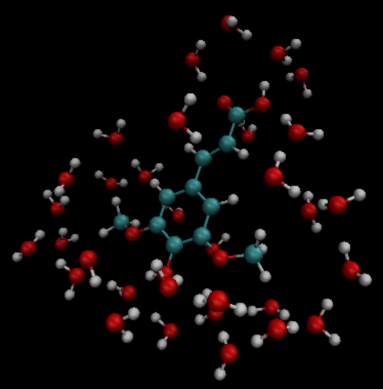
According to the coordinate information in the sa.pdb file, the TDDFT is calculated, and the input file is as follows:

$COMPASS
Title
 SA Molecule test run
Basis
 6-31g
Geometry
C          14.983  14.539   6.274
C          14.515  14.183   7.629
C          13.251  14.233   8.118
C          12.774  13.868   9.480
C          11.429  14.087   9.838
C          10.961  13.725  11.118
O           9.666  13.973  11.525
C           8.553  14.050  10.621
C          11.836  13.125  12.041
O          11.364  12.722  13.262
C          13.184  12.919  11.700
O          14.021  12.342  12.636
C          15.284  11.744  12.293
C          13.648  13.297  10.427
O          14.270  14.853   5.341
O          16.307  14.468   6.130
H          15.310  13.847   8.286
H          12.474  14.613   7.454
H          10.754  14.550   9.127
H           7.627  14.202  11.188
H           8.673  14.888   9.924
H           8.457  13.118  10.054
H          10.366  12.712  13.206
H          15.725  11.272  13.177
H          15.144  10.973  11.525
H          15.985  12.500  11.922
H          14.687  13.129  10.174
H          16.438  14.756   5.181
O          18.736   9.803  12.472
H          18.779  10.597  11.888
H          19.417  10.074  13.139
O          18.022  14.021   8.274
H          17.547  14.250   7.452
H          18.614  13.310   7.941
O           8.888  16.439   7.042
H           9.682  16.973   6.797
H           8.217  17.162   7.048
O           4.019  14.176  11.140
H           4.032  13.572  10.360
H           4.752  14.783  10.885
O          16.970   8.986  14.331
H          17.578   9.273  13.606
H          17.497   8.225  14.676
O           8.133  17.541  10.454
H           8.419  17.716  11.386
H           8.936  17.880   9.990
O           8.639  12.198  13.660
H           7.777  11.857  13.323
H           8.413  13.155  13.731
O          13.766  11.972   4.742
H          13.858  12.934   4.618
H          13.712  11.679   3.799
O          10.264  16.103  14.305
H           9.444  15.605  14.054
H          10.527  15.554  15.084
O          13.269  16.802   3.701
H          13.513  16.077   4.325
H          14.141  17.264   3.657
O          13.286  14.138  14.908
H          13.185  14.974  14.393
H          13.003  13.492  14.228
O          16.694  11.449  15.608
H          15.780  11.262  15.969
H          16.838  10.579  15.161
O           7.858  14.828  14.050
H           7.208  15.473  13.691
H           7.322  14.462  14.795
O          15.961  17.544   3.706
H          16.342  16.631   3.627
H          16.502  17.866   4.462
O          10.940  14.245  16.302
H          10.828  13.277  16.477
H          11.870  14.226  15.967
O          12.686  10.250  14.079
H          11.731  10.151  14.318
H          12.629  11.070  13.541
O           9.429  11.239   8.483
H           8.927  10.817   7.750
H           9.237  12.182   8.295
O          17.151  15.141   3.699
H          17.124  14.305   3.168
H          18.133  15.245   3.766
O          17.065  10.633   9.634
H          16.918  10.557   8.674
H          17.024   9.698   9.909
O          17.536  14.457  10.874
H          18.014  13.627  11.089
H          17.683  14.460   9.890
O           5.836  16.609  13.299
H           4.877  16.500  13.549
H           5.760  16.376  12.342
O          19.014  12.008  10.822
H          18.249  11.634  10.308
H          19.749  11.655  10.256
O          15.861  14.137  15.750
H          14.900  13.990  15.574
H          16.185  13.214  15.645
O          11.084   9.639  10.009
H          11.641   9.480   9.213
H          10.452  10.296   9.627
O          14.234  10.787  16.235
H          13.668  10.623  15.444
H          13.663  10.376  16.925
O          14.488   8.506  13.105
H          13.870   9.136  13.550
H          15.301   8.683  13.628
O          14.899  17.658   9.746
H          15.674  18.005   9.236
H          15.210  16.754   9.926
O           8.725  13.791   7.422
H           9.237  13.488   6.631
H           8.845  14.770   7.309
O          10.084  10.156  14.803
H           9.498  10.821  14.366
H          10.215  10.613  15.669
O           5.806  16.161  10.582
H           5.389  16.831   9.993
H           6.747  16.470  10.509
O           6.028  13.931   7.206
H           5.971  14.900   7.257
H           6.999  13.804   7.336
O          17.072  12.787   2.438
H          16.281  12.594   1.885
H          17.062  11.978   3.013
END geometry
nosymm
mpec+cosx
$END

$xuanyuan
$end

$SCF
rks
dft
 b3lyp
solvent
 water
grid
 medium
$END

# input for tddft
$tddft
iroot    # Calculate 1 root for each irrep. By default, 10 roots are calculated
  1      # for each irrep
memjkop  # maxium memeory for Coulomb and Exchange operator. 1024 MW (Mega Words)
  1024
$end

A list of solvent types supported in BDF

Name	Short Name	${\epsilon}$	${\epsilon_{opt}}$
water	H2O	78.3553	1.7764
acetic acid	ACETACID	6.2528	1.8824
acetone	ACETONE	20.4930	1.8463
acetonitrile	ACETNTRL	35.6880	1.8069
acetophenone	ACETPHEN	17.4400	2.3630
aniline	ANILINE	6.8882	2.5163
anisole	ANISOLE	4.2247	2.3025
benzaldehyde	BENZALDH	18.2200	2.3910
benzene	BENZENE	2.2706	2.2533
benzonitrile	BENZNTRL	25.5920	2.3375
benzyl chloride	BENZYLCL	6.7175	2.3688
1-bromo-2-methylpropane	BRISOBUT	7.7792	2.0587
bromobenzene	BRBENZEN	5.3954	2.4327
bromoethane	BRETHANE	9.0100	2.0275
bromoform	BROMFORM	4.2488	2.5616
1-bromooctane	BROCTANE	5.0244	2.1095
1-bromopentane	BRPENTAN	6.2690	2.0872
2-bromopropane	BRPROPA2	9.3610	2.0309
1-bromopropane	BRPROPAN	8.0496	2.0572
butanal	BUTANAL	13.4500	1.9163
butanoic acid	BUTACID	2.9931	1.9544
1-butanol	BUTANOL	17.3320	1.9580
2-butanol	BUTANOL2	15.9440	1.9538
butanone	BUTANONE	18.2460	1.9011
butanonitrile	BUTANTRL	24.2910	1.9160
butyl acetate	BUTILE	4.9941	1.9435
butylamine	NBA	4.6178	1.9687
n-butylbenzene	NBUTBENZ	2.3600	2.2195
sec-butylbenzene	SBUTBENZ	2.3446	2.2186
tert-butylbenzene	TBUTBENZ	2.3447	2.2282
carbon disulfide	CS2	2.6105	2.6631
carbon tetrachloride	CARBNTET	2.2280	2.1319
chlorobenzene	CLBENZEN	5.6968	2.3229
sec-butyl chloride	SECBUTCL	8.3930	1.9519
chloroform	CHCL3	4.7113	2.0906
1-chlorohexane	CLHEXANE	5.9491	2.0161
1-chloropentane	CLPENTAN	6.5022	1.9957
1-chloropropane	CLPROPAN	8.3548	1.9263
o-chlorotoluene	OCLTOLUE	4.6331	2.3311
m-cresol	M-CRESOL	12.4400	2.3833
o-cresol	O-CRESOL	6.7600	2.3596
cyclohexane	CYCHEXAN	2.0165	2.0352
cyclohexanone	CYCHEXON	15.6190	2.1045
cyclopentane	CYCPENTN	1.9608	1.9782
cyclopentanol	CYCPNTOL	16.9890	2.1112
cyclopentanone	CYCPNTON	13.5800	2.0638
cis-decalin	DECLNCIS	2.2139	2.1934
trans-decalin	DECLNTRA	2.1781	2.1594
decalin (cis/trans mixture)	DECLNMIX	2.1960	2.1765
n-decane	DECANE	1.9846	1.9887
1-decanol	DECANOL	7.5305	2.0655
1,2-dibromoethane	EDB12	4.9313	2.3676
dibromomethane	DIBRMETN	7.2273	2.3778
dibutyl ether	BUTYLETH	3.0473	1.9578
o-dichlorobenzene	ODICLBNZ	9.9949	2.4072
1,2-dichloroethane	EDC12	10.1250	2.0874
cis-dichloroethylene	C12DCE	9.2000	2.0996
trans-dichloroethylene	T12DCE	2.1400	2.0892
dichloromethane	DCM	8.9300	2.0283
diethyl ether	ETHER	4.2400	1.8295
diethyl sulfide	ET2S	5.7230	2.0822
diethylamine	DIETAMIN	3.5766	1.9221
diiodomethane	MI	5.3200	3.0363
diisopropyl ether	DIPE	3.3800	1.8712
dimethyl disulfide	DMDS	9.6000	2.3375
dimethyl sulfoxide	DMSO	46.8260	2.0079
n,n-dimethylacetamide	DMA	37.7810	2.0678
cis-1,2-dimethylcyclohexane	CISDMCHX	2.0600	2.0621
n,n-dimethylformamide	DMF	37.2190	2.0463
2,4-dimethylpentane	DMEPEN24	1.8939	1.9085
2,4-dimethylpyridine	DMEPYR24	9.4176	2.2530
2,6-dimethylpyridine	DMEPYR26	7.1735	2.2359
1,4-dioxane	DIOXANE	2.2099	2.0232
diphenyl ether	PHOPH	3.7300	2.4923
dipropylamine	DPROAMIN	2.9112	1.9740
n-dodecane	DODECAN	2.0060	2.0209
1,2-ethanediol	MEG	40.2450	2.0501
ethanethiol	ETSH	6.6670	2.0478
ethanol	ETHANOL	24.8520	1.8526
ethyl acetate	ETOAC	5.9867	1.8832
ethyl formate	ETOME	8.3310	1.8493
ethylbenzene	EB	2.4339	2.2377
ethylphenyl ether	PHENETOL	4.1797	2.2729
fluorobenzene	C6H5F	5.4200	2.1562
1-fluorooctane	FOCTANE	3.8900	1.9418
formamide	FORMAMID	108.9400	2.0944
formic acid	FORMACID	51.1000	1.8807
n-heptane	HEPTANE	1.9113	1.9260
1-heptanol	HEPTANOL	11.3210	2.0303
2-heptanone	HEPTNON2	11.6580	1.9847
4-heptanone	HEPTNON4	12.2570	1.9794
n-hexadecane	HEXADECN	2.0402	2.0578
n-hexane	HEXANE	1.8819	1.8904
hexanoic acid	HEXNACID	2.6000	2.0059
1-hexanol	HEXANOL	12.5100	2.0102
2-hexanone	HEXANON2	14.1360	1.9620
1-hexene	HEXENE	2.0717	1.9146
1-hexyne	HEXYNE	2.6150	1.9569
iodobenzene	C6H5I	4.5470	2.6244
1-iodobutane	IOBUTANE	6.1730	2.2503
iodoethane	C2H5I	7.6177	2.2901
1-iodohexadecane	IOHEXDEC	3.5338	2.1922
iodomethane	CH3I	6.8650	2.3654
1-iodopentane	IOPENTAN	5.6973	2.2377
1-iodopropane	IOPROPAN	6.9626	2.2674
isopropylbenzene	CUMENE	2.3712	2.2246
p-isopropyltoluene	P-CYMENE	2.2322	2.2228
mesitylene	MESITYLN	2.2650	2.2482
methanol	METHANOL	32.6130	1.7657
2-methoxyethanol	EGME	17.2000	1.9667
methyl acetate	MEACETAT	6.8615	1.8534
methyl benzoate	MEBNZATE	6.7367	2.2995
methyl butanoate	MEBUTATE	5.5607	1.9260
methyl formate	MEFORMAT	8.8377	1.8045
4-methyl-2-pentanone	MIBK	12.8870	1.9494
methyl propanoate	MEPROPYL	6.0777	1.8975
2-methyl-1-propanol	ISOBUTOL	16.7770	1.9474
2-methyl-2-propanol	TERBUTOL	12.4700	1.9260
n-methylaniline	NMEANILN	5.9600	2.4599
methylcyclohexane	MECYCHEX	2.0240	2.0252
n-methylformamide (E/Z mixture)	NMFMIXTR	181.5600	2.0503
2-methylpentane	ISOHEXAN	1.8900	1.8810
2-methylpyridine	MEPYRID2	9.9533	2.2371
3-methylpyridine	MEPYRID3	11.6450	2.2620
4-methylpyridine	MEPYRID4	11.9570	2.2611
nitrobenzene	C6H5NO2	34.8090	2.4218
nitroethane	C2H5NO2	28.2900	1.9368
nitromethane	CH3NO2	36.5620	1.9091
1-nitropropane	NTRPROP1	23.7300	1.9650
2-nitropropane	NTRPROP2	25.6540	1.9444
o-nitrotoluene	ONTRTOLU	25.6690	2.3870
n-nonane	NONANE	1.9605	1.9751
1-nonanol	NONANOL	8.5991	2.0543
5-nonanone	NONANONE	10.6000	2.0150
n-octane	OCTANE	1.9406	1.9527
1-octanol	OCTANOL	9.8629	2.0435
2-octanone	OCTANON2	9.4678	2.0025
n-pentadecane	PENTDECN	2.0333	2.0492
pentanal	PENTANAL	10.0000	1.9444
n-pentane	NPENTANE	1.8371	1.8428
pentanoic acid	PENTACID	2.6924	1.9839
1-pentanol	PENTANOL	15.1300	1.9884
2-pentanone	PENTNON2	15.2000	1.9307
3-pentanone	PENTNON3	16.7800	1.9388
1-pentene	PENTENE	1.9905	1.8810
E-2-pentene	E2PENTEN	2.0510	1.9025
pentyl acetate	PENTACET	4.7297	1.9664
pentylamine	PENTAMIN	4.2010	2.0967
perfluorobenzene	PFB	2.0290	1.8981
phenylmethanol	BENZALCL	12.4570	2.3704
propanal	PROPANAL	18.5000	1.8594
propanoic acid	PROPACID	3.4400	1.9235
1-propanol	PROPANOL	20.5240	1.9182
2-propanol	PROPNOL2	19.2640	1.8978
propanonitrile	PROPNTRL	29.3240	1.8646
2-propen-1-ol	PROPENOL	19.0110	1.9980
propyl acetate	PROPACET	5.5205	1.9160
propylamine	PROPAMIN	4.9912	1.9238
pyridine	PYRIDINE	12.9780	2.2786
tetrachloroethene	C2CL4	2.2680	2.2659
tetrahydrofuran	THF	7.4257	1.9740
tetrahydrothiophene-s,s-dioxide	SULFOLAN	43.9620	2.2002
tetralin	TETRALIN	2.7710	2.3756
thiophene	THIOPHEN	2.7270	2.3375
thiophenol	PHSH	4.2728	2.5259
toluene	TOLUENE	2.3741	2.2383
tributyl phosphate	TBP	8.1781	2.0232
1,1,1-trichloroethane	TCA111	7.0826	2.0676
1,1,2-trichloroethane	TCA112	7.1937	2.1650
trichloroethene	TCE	3.4220	2.1824
triethylamine	ET3N	2.3832	1.9628
2,2,2-trifluoroethanol	TFE222	26.7260	1.6659
1,2,4-trimethylbenzene	TMBEN124	2.3653	2.2644
2,2,4-trimethylpentane	ISOCTANE	1.9358	1.9363
n-undecane	UNDECANE	1.9910	2.0730
m-xylene	M-XYLENE	2.3478	2.2416
o-xylene	O-XYLENE	2.5454	2.2665
p-xylene	P-XYLENE	2.2705	2.2374
xylene (mixture)	XYLENEMX	2.3879	2.2485
1,1-dichloroethane		10.1900	2.0880
1-iodopentene		5.7800	2.2350
1-pentyne		2.0600	1.9182
2-chlorobutane		8.3900	1.9656
benzyl alcohol		11.9200	2.3716
bromooctane		5.0200	2.1083
butyl ethanoate		5.0700	1.9432
butyl benzene		2.3600	2.2201
carbon tet		2.2300	2.1316
chlorotoluene		6.8500	2.3654
decalin		2.1900	2.1934
dimethylacetamide	DMAC	37.7800	2.0678
dimethylformamide	DMF	37.2200	2.0478
dimethylpyridine		7.1700	2.2350
dodecane		2.0100	2.0221
E-1,2-dichloroethene		2.1400	2.0880
ethyl ethanoate		6.0800	1.8824
ethyl methanoate		8.3300	1.8469
ethyl eneglycol		40.2500	2.0506
hexadecyl iodide		3.5300	2.1934
hexanoic		2.6000	2.0051
isobutanol		16.7800	1.9460
isopropyl ether		3.8800	1.8714
isopropyl toluene		2.2300	2.2231
methyl ethanoate		6.8600	1.8523
methyl methanoate		8.8400	1.8036
methyl phenyl ketone		17.4400	2.3624
methylformamide		181.5600	2.0506
hexadecane		2.0600	2.0592
methylaniline		5.9600	2.4649
pentane		1.8400	1.8414
pentadecane		2.0300	2.0478
pentyl ethanoate		4.7300	1.9656
phenyl ether		3.7300	2.4932
propyl ethanoate		5.5200	1.9155
pyrrolidine		8.0400	2.0822
sec-butanol		15.9400	1.9544
t-butanol		12.4700	1.9238
t-butylbenzene		2.3400	2.2290
tetrahyrothiophenedioxide		43.9600	2.1993
tribromomethane		4.2500	2.5632
trichloromethane	TCM	4.7100	2.0909
Z-1,2-dichloroethene		9.2000	2.0996
isoquinoline		11.0000	1.0100
quinoline		9.1600	1.0100
diethylether		4.2400	1.8295
dichloroethane		10.1250	2.0874
carbontetrachloride		2.2280	2.1319
heptane		1.9113	1.9260
dimethylsulfoxide		46.8260	2.0079
argon		1.4300	1.4300
krypton		1.5190	1.5190
xenon		1.7060	1.7060
n-octanol		9.8629	2.0435
aceticacid		6.2528	1.8824
a-chlorotoluene		6.7175	2.3688
benzylalcohol		12.4570	2.3704
butanoicacid		2.9931	1.9544
butylethanoate		4.9941	1.9435
carbondisulfide		2.6105	2.6631
decalin-mixture		2.1960	2.1106
dibutylether		3.0473	1.9578
diethylsulfide		5.7230	2.0822
diisopropylether		3.3800	1.8712
dimethyldisulfide		9.6000	2.3375
diphenylether		3.7300	2.4923
E-1,2-dichloroethene		2.1400	2.0892
E-2-pentene		2.0510	1.9025
ethylethanoate		5.9867	1.8832
ethylmethanoate		8.3310	1.8493
ethylphenylether		4.1797	2.2729
formicacid		51.1000	1.8807
hexanoicacid		2.6000	2.0059
methylbenzoate		6.7367	2.2995
methylbutanoate		5.5607	1.9260
methylethanoate		6.8615	1.8534
methylmethanoate		8.8377	1.8045
methylpropanoate		6.0777	1.8975
n-methylaniline		5.9600	2.4599
n-methylformamide-mixture		181.5600	2.0503
n,n-dimethylacetamide		37.7810	2.0678
n,n-dimethylformamide		37.2190	2.0463
pentanoicacid		2.6924	1.9839
pentylethanoate		4.7297	1.9664
propanoicacid		3.4400	1.9235
propylethanoate		5.5205	1.9160
tetrahydrothiophene-s,s-dioxide		43.9620	2.2002
tributylphosphate		8.1781	2.0232
xylene-mixture		2.3879	2.2485
Z-1,2-dichloroethene		9.2000	2.0996

Point Charge Model

BDF supports incorporating MM region atomic charges as point charges in calculations. Point charges are input through a file named $BDFTASK.extcharge (same name as the calculation task). The format is as follows:

$COMPASS
Title
water molecule in background of external charges
Basis
  6-31g
Geometry
O   0.000000   0.000000   0.106830
H   0.000000   0.785178  -0.427319
H   0.000000  -0.785178  -0.427319
End Geometry
Extcharge  # Indicates point charges will be input
  point      # Specifies point charge type
$END

$XUANYUAN
$END

$SCF
RHF
$END

Point charge input file (e.g., h2o.extcharge):

External charge, Point charge   # Header/description line
6                               # Number of point charges
C1     -0.732879     0.000000     5.000000     0.114039  # Label, x, y, z, charge
C2      0.366440     0.000000     5.780843    -0.456155
C3      0.366440     0.000000     4.219157    -0.456155
C4     -0.732879     0.000000    10.000000     0.114039
C5      0.366440     0.000000    10.780843    -0.456155
C6      0.366440     0.000000     9.219157    -0.456155

Default Format: Atom_label x y z Charge Coordinates default to Angstrom units.

Bohr Units Format: Specify units in the second line:

External charge, Point charge
6    Bohr                      # Unit: Bohr
C1     -0.732879    0.000000    5.000000    0.114039

# omitted #

Wavefunction Analysis and Property Analysis

The solutions to the Schrödinger equation consist of two parts: the wavefunction (eigenvector) and the energy (eigenvalue). Both can be utilized for various subsequent analyses to establish connections with chemical concepts and experimental observables. These analysis methods fall into three categories: wavefunction analysis related to the wavefunction itself, density analysis related to the electron density (i.e., the square modulus of the wavefunction), and various one-electron properties related to energy derivatives.

BDF supports the following wavefunction analyses: * Mulliken population analysis and Löwdin population analysis, including atomic net charges and atomic spin densities.

BDF supports the following one-electron properties:

SCF: Dipole moment, Polarizability*, Hyperpolarizability*, Mössbauer spectroscopy (Effective Contact Density, Electric Field Gradient), Nuclear Magnetic Resonance**
TDDFT: Dipole moment of excited states*, Oscillator strength for fluorescence absorption spectra, Oscillator strength for phosphorescence absorption spectra

* Calculated in the resp module. ** Calculated in the nmr module.

Additional wavefunction analyses, density analyses, and one-electron properties can be performed using third-party programs by generating molden-format data files in the scf module. Input example:

$scf
rks
dft
 b3lyp
molden
$end

The standard molden format only supports spdfg-type Gaussian basis functions, but BDF has extended support to include h functions.

Effective Contact Density

Calculating the Effective Contact Density (ED) requires consideration of both relativistic effects (handled in BDF using the X2C Hamiltonian via heff = 21, 22, or 23) and the finite size of the nucleus (nuclear = 1). An input example at the sf-X2C-AU/B3LYP level is:

$xuanyuan
 heff
  23
 nuclear
  1
$end

$scf
 rks
 dft
  b3lyp
 grid
  ultra fine
 reled
  20
$end

Here, reled invokes the relativistic property ED calculation. 20 specifies that ED is not calculated for light elements with atomic numbers less than 20, saving computational time. For density functional calculations, the ED value is sensitive to the integration grid; it is recommended to use the fine-grid setting ultra fine.

Special basis set treatment is required for ED; see Mössbauer Spectrum.

Electric Field Gradient

Calculating the Electric Field Gradient (EFG) has similar requirements to ED and uses the keyword relefg. See Mössbauer Spectrum.

molden2aim

Download: https://github.com/zorkzou/Molden2AIM

molden2aim converts molden files generated by BDF into wfn, wfx, or NBO-47 format data files for various analyses. It supports spdfgh-type Gaussian basis functions and ECPs.

Multiwfn

Download: http://sobereva.com/multiwfn/

Multiwfn is a powerful wavefunction analysis program. Using molden data files generated by BDF (supporting spdfgh basis functions and ECPs) or wfn/wfx files converted via molden2aim, Multiwfn can perform numerous analyses. These include: * Electron density topological analysis (also known as Quantum Theory of Atoms in Molecules; QTAIM) * Electron Localization Function (ELF) * Population analysis * Bond order analysis * Atomic charge analysis It can also visualize molecular orbitals, electron density, and various real-space functions. Details are in the Multiwfn manual.

NBO Analysis

BDF currently does not include a direct interface to NBO (https://nbo7.chem.wisc.edu/). However, molden2aim can be used to convert BDF-generated molden files (supporting spdfgh basis functions and ECPs) into NBO-47 format data files. These can then be analyzed using the standalone NBO program gennbo.exe.

For RHF/RKS and UHF/UKS type wavefunctions (i.e., MO occupation numbers limited to 0, 1, or 2), NBO can perform “Second Order Perturbation Theory Analysis.” This requires the presence of the Fock matrix in the .47 file. Set nbopro=1 in molden2aim’s configuration file m2a.ini to achieve this.

Force Constants in Internal Coordinates

The Hessian matrix (also called the force constant matrix) produced by vibrational frequency calculations represents the second derivative of energy with respect to the 3N Cartesian coordinates of the atoms. Chemically, however, force constants in internal coordinates (e.g., chemical bonds, bond angles, dihedral angles) are often more relevant. Third-party programs can “extract” force constants for internal coordinates from the Hessian matrix. These are useful for parameterizing molecular mechanics (MM) calculations or comparing the strengths of chemical bonds and hydrogen bonds. A theoretical introduction in Chinese is available at: http://bbs.keinsci.com/thread-28658-1-1.html

LModeA: Standalone program written in Fortran90. Requires application to Elfi Kraka: https://s3.smu.edu/dedman/catco/members.html
LModeA-nano: A PyMOL plugin supporting local vibrational mode analysis for solids and molecules, calculating force constants and harmonic frequencies for bonds, angles, etc.: https://lmodea-nano.readthedocs.io/en/latest/
Morfeus: Standalone program written in Python: https://digital-chemistry-laboratory.github.io/morfeus/index.html

The .umv data file generated by BDF vibrational frequency calculations can be read directly by these programs.

Energy Decomposition Analysis

Benefiting from BDF’s automatic fragmentation engine autofrag, since June 2025, BDF supports energy decomposition analysis for covalent or non-covalent complexes based on sobEDA and sobEDAw methods [69].

In the sobEDA method, given a system XY, the program can automatically divide XY into two fragments X and Y according to the bonding relationship, and then perform calculations on X and Y separately. Then, it combines the local orbitals of X and Y, calculates the electrostatic interaction energy Eels, exchange interaction energy Ex, DFT-related interaction energy Edftc, dispersion correction contribution Edc, solvent correction contribution Esolv, etc. Next, it performs Löwdin orthogonalization on the local orbitals of X and Y, and performs SCF iteration until convergence. The two-step energy change can also obtain the Pauli repulsion energy Erep and orbital interaction energy Eorb. Thus, the interaction energy between X and Y is decomposed into a sum of contributions from different sources. Here, X and Y can not only be two complete molecules (i.e., they have only non-covalent interactions), but also two fragments that are bonded to each other. There can even be more than one covalent/coordinate bond between the fragments, but in this case, the fragments must be open-shell, i.e., the broken bonds must be treated as free radicals rather than being saturated with buffer atoms/hydrogen atoms/PHO atoms. The program can also analyze systems consisting of more than two fragments, but regardless of whether it is Eels, Ex, Edftc, Edc, Esolv, Erep, or Eorb, only the total contribution of all fragment pairs can be obtained, and not the interaction energy of a specific pair of fragments. In the sobEDAw method, based on the sobEDA analysis, the program further allocates Edftc to Edc and Ex in a certain proportion, and the resulting value can serve as an approximation of the SAPT energy decomposition analysis result, but sobEDAw is only suitable for analyzing non-covalent interactions.

Compared to other energy decomposition analysis methods, sobEDA and sobEDAw have the following advantages:

The computation cost is relatively low, similar to that of a single-point DFT energy calculation for the whole system, and is 1-2 orders of magnitude faster than LED, SAPT, etc.;
The sum of various terms obtained from energy decomposition analysis is strictly equal to the interaction energy between two fragments;
The physical meaning of the decomposition result is clear.

In addition, the sobEDA and sobEDAw methods implemented in BDF have the following extra advantages over the original sobEDA and sobEDAw methods:

As a byproduct of the calculation, localized molecular orbitals (LMOs) for fragments and the total system can be obtained, which can be visualized or further analyzed;
When analyzing non-covalent interactions, the program can automatically identify which molecules make up the system without manually specifying atomic numbers;
Supports a subset of range-separated functionals (CAM-B3LYP, LC-BLYP);
Can analyze the contribution of solvent to interaction energy.

On the other hand, the sobEDA and sobEDAw methods (or their BDF implementations) also have some limitations:

Does not take into account the deformation energy of fragments (the energy increase brought about by the fragment changing from its equilibrium structure to its structure in the complex), as well as the contributions of zero-point energy, enthalpy correction and entropy correction. Users who need these contributions should calculate them manually according to their definitions;
sobEDA only has meaningful results when used with theoretical levels such as B3LYP-D3 that combine a functional without dispersion correction + dispersion correction. sobEDAw does not have this limitation, but to avoid self-fitting empirical parameters as much as possible, it is still recommended to use GB3LYP-D3 unless there are special requirements;
sobEDAw involves three empirical parameters (c, a, r) related to the theoretical level, and there are limited theoretical levels that have been fitted with these parameters in the literature; if used in conjunction with other theoretical levels, the parameters need to be fitted manually;
BDF implements sobEDA and sobEDAw methods that do not currently support composite basis (CB) calculations;
BDF implements sobEDA and sobEDAw methods for a limited set of functionals; see the section on “Exchange-Correlation Functionals Supported in BDF” in the User Guide for details. Note that “support” here does not mean the program can automatically select the correct sobEDAw empirical parameters, so users usually still need to manually input these parameters.

sobEDA example: Analyzing the interaction energy between two HC groups in acetylene

This example comes from Table 5 of the original literature sobEDA [69]:

$autofrag
method
sobeda
fragdef
0 4 0 -4 # charge1 spinmult1 charge2 spinmult2. Negative spinmult indicates beta spins
1,2 # fragment 1: atom 1,2 (HC)
3,4 # fragment 2: atom 3,4 (CH)
$end

$compass
title
  sobEDA analysis of acetylene (GB3LYP-D3/def2-TZVP)
geometry
      H          -0.00000000      -0.00000000       1.66144913
      C          -0.00000000      -0.00000000       0.59846873
      C           0.00000000       0.00000000      -0.59846873
      H           0.00000000       0.00000000      -1.66144913
end geometry
basis
def2-TZVP # for non-covalent complexes, diffuse basis sets (e.g. def2-TZVPD) are recommended
mpec+cosx # not necessary for molecules of this size, but helpful for large systems
$end

$xuanyuan
$end

$scf
# even if the total system is closed-shell, if some of the fragments
# are open-shell, one should still write UKS instead of RKS here
uks
dft
gb3lyp
d3 # dispersion correction is necessary for sobEDA. "D3" defaults to B-J damping, not zero damping
$end

$localmo
flmo # necessary even if the user does not need LMOs
$end

Note that since HC is a shell layer, it is necessary to specify which atoms each fragment contains using the fragdef keyword in the autofrag module (otherwise, the program does not know which bond(s) to break), as well as the charge and spin multiplicity of each fragment. The atomic numbers of each fragment are separated by commas, and consecutive atomic numbers can be written in the form “start number-end number”, such as “1,3,6-10,12-13,15” is equivalent to “1,3,6,7,8,9,10,12,13,15”. Although the ground state of HC is a doublet, the triple bond formed between the two HC groups requires exciting HC to a quartet state, so the energy decomposition analysis is performed based on the quartet state HC. The spin multiplicity of the second HC fragment is written as -4 instead of 4 to indicate that its single-electron spin direction is opposite to that of the first fragment (with positive spin multiplicity). If analyzing non-covalent complexes, i.e., cases where the program can complete fragmentation without breaking any bonds, fragdef does not need to be specified, but users must check whether the fragments and spin multiplicities automatically identified by the program are reasonable; if not, they still need to use the fragdef keyword to specify the charge and spin multiplicity of each fragment, as well as their atomic composition.

The program first calls the autofrag module for fragmentation and then performs SCF calculations on the two fragments in sequence, with results output to *.fragment1.out and *.fragment2.out respectively; the local orbitals (LMO) of the fragments are output to *.fragment1.flmo.molden and *.fragment2.flmo.molden, which can be opened by any orbital visualization software that supports the molden format. Next, the program performs three global SCF calculations: the first does not orthogonalize pFLMO or perform SCF iterations; the second orthogonalizes pFLMO but does not perform SCF iterations; and the third both orthogonalizes pFLMO and performs SCF iterations until convergence. Finally, the program integrates the results of the five calculations and outputs energy decomposition analysis results:

    *** Energy decomposition analysis result ***
Total interaction      energy:   -275.837 kcal/mol
Of these:
 - Electrostatic       energy:   -143.258 kcal/mol
 - Exchange-repulsion  energy:    248.908 kcal/mol
   Of these:
    > Exchange         energy:    -58.637 kcal/mol
    > Repulsion        energy:    307.545 kcal/mol
 - Orbital interaction energy:   -336.724 kcal/mol
 - Correlation         energy:    -44.763 kcal/mol
   Of these:
    > DFT correlation        :    -43.872 kcal/mol
    > Dispersion correction  :     -0.891 kcal/mol
 - Implicit solvation  energy:      0.000 kcal/mol

Among them: * Electrostatic energy refers to electrostatic potential energy; for this system, the electrostatic potential energy is a very large negative absolute value, because the two carbon atoms are very close, and the electron cloud of one carbon atom will penetrate into the interior of the electron cloud of another carbon atom, feeling the nuclear attraction of the latter. * Exchange-repulsion energy refers to the exchange-repulsion energy, which can be used to characterize the contribution of steric hindrance. At first glance, acetylene as a very small molecule has no steric hindrance, but this is because only in cases where non-covalent interactions have a smaller contribution to orbital effects, the exchange-repulsion energy can dominate and manifest as steric repulsion; when studying the direct bonding of two atoms, there is indeed steric hindrance between the atoms, it’s just that the orbital effect is more significant than the steric contribution, leading to many cases where the contribution of steric hindrance to covalent bonds is not discussed. * Orbital interaction energy refers to the orbital effect energy, which has a large absolute negative value for covalent bonds and a relatively small absolute value for non-covalent interactions. This term represents the contributions of covalent effects, polarization effects, and charge transfer effects to the interaction energy. Note that the boundaries between these three contributions are blurred and may even overlap, so it is not possible to further decompose the orbital effect energy into covalent, polarizing, and charge transfer contributions within the sobEDA framework. * Correlation energy refers to electron correlation energy, which includes contributions from the functional’s own electron correlation energy (DFT correlation) and dispersion correction. For functionals such as B3LYP that cannot describe dispersion effects, the dispersion correction contribution obtained by sobEDA can be considered as the contribution of dispersion energy to interaction energy. However, note that the absolute value of the dispersion energy obtained in this way is often smaller than that obtained from some high-level energy decomposition analysis methods (such as LED, SAPT), and the difference is often even more pronounced for covalently bonded systems due to the non-uniqueness of the definition of dispersion energy at short inter-fragment distances [70] , which does not imply that sobEDA’s results are unreliable. To obtain results comparable to those from LED and SAPT, one should use sobEDAw (see below). * Implicit solvation energy refers to the contribution of implicit solvent models to the interaction energy; for calculations without an implicit solvent model, this term is exactly 0 (even if the user adds explicit solvent with QM or MM). Note that when users consider non-electrostatic terms of solvent models or use SMD solvent models, this term includes entropy contributions from solvation and should be referred to as the contribution of dissolution free energy (rather than solvation energy) to interactions.

It can be seen that sobEDA can not only be used to analyze non-covalent compounds and fragments connected by single bonds, but also to analyze fragments connected by multiple bonds. Similarly, the bonds formed between fragments are not limited to one. However, when there are covalent/coordinate bonds between fragments, users must take into account the unpaired electrons introduced by bond breaking when defining the spin multiplicity of the fragments, and even check whether the fragments have converged to the correct wave function (e.g., through spin population analysis), simply confirming that the parity of the spin multiplicity is correct is not enough.

If the keyword molden is added to the $scf block in the above input file, the pFLMO orbitals and FLMO orbitals of the total system can also be generated, which are *.global.pflmo.molden and *.global.cflmo.molden respectively. This allows for a comparison of the LMOs with pFLMOs and FLMOs of molecular fragments. The difference in shape between LMO and pFLMO represents the effect of orbital orthogonalization, corresponding to the exchange energy in the above energy decomposition analysis; the difference in shape between pFLMO and FLMO represents the effect of inter-fragment orbital mixing, corresponding to the orbital interaction energy in the above energy decomposition analysis. For example, the following figure shows the shape change process of a p-orbital of HC in the above example, where it can be seen that orbital orthogonalization causes LMO to shrink slightly away from another fragment, while orbital mixing causes LMO to delocalize towards another fragment. The calculated FLMO is not a pure pi-orbital but contains a small amount of sigma component, which is normal. Adding the pipek keyword in the $localmo module can often help obtain pure sigma and pi orbitals by using Pipek-Mezey localization, but still cannot strictly guarantee that sigma and pi do not mix.

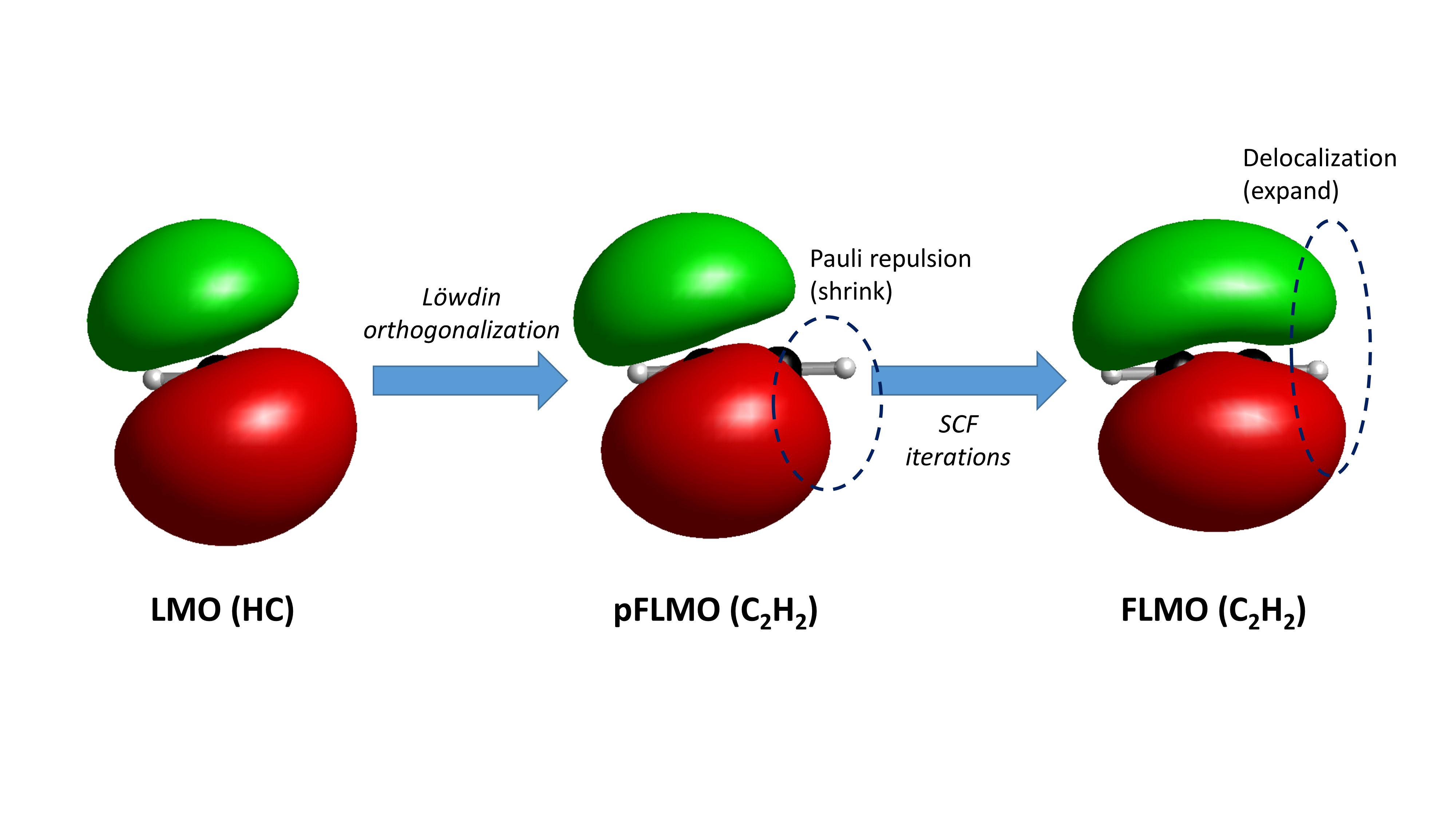
sobEDAw Example: Water Dimer Energy Decomposition Analysis

For non-covalent complexes that are not affected by the limitations described at the beginning of this chapter, it is recommended to use sobEDAw instead of sobEDA for energy decomposition analysis. For example, the following input file decomposes the interaction energy between two water molecules in a water dimer in liquid water environment, taking into account the contribution of surrounding water molecules using an implicit solvent model:

$autofrag
method
sobedaw
# parameters for GB3LYP/6-31+G(d,p)
# JPCA, 2023, 127, 7023
# Note that this is a rather poor level of theory for sobEDAw;
# for accurate results, diffuse TZ basis sets are recommended
sobedaw_c
0.638
sobedaw_a
0.124
sobedaw_r
3.523
$end

$compass
geometry
   O         -1.65542061     -0.12330038      0.00000000
   O          1.24621244      0.10268870      0.00000000
   H         -0.70409026      0.03193167      0.00000000
   H         -2.03867273      0.75372294      0.00000000
   H          1.57598558     -0.38252146     -0.75856129
   H          1.57598558     -0.38252146      0.75856129
end geometry
basis
6-31+G(d,p)
$end

$xuanyuan
$end

$scf
rks
dft
gb3lyp
d3
solvent
water
$end

$localmo
flmo
$end

It can be seen that the parameters c, a, and r required by sobEDAw need to be looked up from the original literature of sobEDA or fitted manually. The analysis result is

sobEDAw parameters:
c = 0.63800000
a = 0.12400000
r = 3.52300000
dEdc/dEels = 0.05722559
w = 1.00000000

    *** Energy decomposition analysis result ***
Total interaction      energy:     -4.775 kcal/mol
Of these:
 - Electrostatic       energy:    -11.166 kcal/mol
 - Exchange-repulsion  energy:      9.531 kcal/mol
 - Orbital interaction energy:     -2.801 kcal/mol
 - Dispersion          energy:     -2.964 kcal/mol
 - Implicit solvation  energy:      2.625 kcal/mol

It can be seen that sobEDAw does not separately print the exchange energy and repulsion energy, nor does it print DFT-related energies. This is because sobEDAw distributes the DFT-related energies in a certain proportion to the exchange-repulsion energy and dispersion energy. From the results of energy analysis, it can be found that electrostatic interaction is the main reason why water molecules can form dimers, but most of the contribution from electrostatic attraction is offset by steric repulsion; orbital interactions (i.e., the covalent component of hydrogen bonds) and dispersion effects also make a significant contribution to the binding energy between water molecules. Due to the high dielectric constant of water, the liquid water environment has a shielding effect on the electrostatic effects between water molecules, weakening their mutual interaction, so the solventization energy contributes to the interaction energy in the form of repulsion.

When the system consists of three or more molecules, each energy item printed by the program is the sum of all pairwise interactions between molecules. For example, for a system ABC consisting of three molecules A, B, and C, the program can print the total electrostatic energy and total exchange-repulsion energy between all molecules in the system, but cannot print the electrostatic energy or exchange-repulsion energy between molecules A and B specifically. However, due to the characteristics of sobEDA and sobEDAw, when there is no implicit solvent, the total intermolecular electrostatic energy of ABC equals the sum of the electrostatic energies calculated separately for AB, BC, and CA. Therefore, in this case, performing energy decomposition on the AB complex without C can yield the electrostatic energy between A and B. However, for items other than electrostatic energy and exchange energy (note that this does not include exchange-repulsion energy), the sum of contributions calculated separately for AB, BC, and CA is not equal to the total contribution of ABC. In some cases, users may want to decompose the interaction energy between AC as a whole and B; in such cases, use the fragdef keyword to define AC as one fragment and B as another.

Similar to sobEDA, in the sobEDAw method analysis, it is also possible to plot the fragments LMO, pFLMO, FLMO of the system, visually showing the shape change of local orbitals during interaction, which will not be repeated here.

Get started quickly

First Example: RHF Calculation of \(\ce{H2O}\) Molecule

Preparing Input

Executing the Calculation

Analyzing Results

Gaussian Basis Sets

All-Electron Basis Sets

Pseudopotential Basis Sets

## Scalar vs. Spin-Orbit Coupling Pseudopotentials

## Aliases and Abbreviations for Standard Basis Sets

## Custom Basis Set Files

Custom Basis Set Files

Assignment of the basis set

Auxiliary basis set

Exchange-Correlation Functionals Supported in BDF

Self-consistent field methods: Hartree-Fock and Kohn-Sham

Restricted Hartree-Fock method (RHF)

Unrestricted Hartree-Fock method (UHF)

Restricted open-shell Hartree-Fock method (ROHF)

RKS, UKS, and ROKS calculations

Kohn-Sham calculations based on RS hybrid functionals

Customize the exact HF-exchange term in hybrid functionals, double hybrid functionals

Dispersion correction for weak interactions

Improve the accuracy of the integration grid of Kohn-Sham calculations

Symmetry and Molecular Point Groups

Ordering of Irreducible Representations

Standard Orientation

Other techniques for self-consistent field calculations

Initial guess of the self-consistent field calculation

Read into the initial guess track

Transfer molecular orbitals with other quantum chemistry procedures

Extend the small base group convergence orbit to a large base group initial guess

The maximal occupancy of molecular orbitals (MOM) method calculates the excited states

Deal with the non-convergence problem of self-consistent field calculations

Acceleration algorithm for self-consistent field computing

iOI-SCF calculation and FLMO method for large systems

Computation of Fragmented Localized Molecular Orbital FLMO (Manual Sharding)

Calculation of Open Shell Singlet State Using FLMO (Automatic Sharding)

iOI-SCF Method

Time-dependent density functional theory

Calculation of closed shell system: R-TDDFT

Calculation of open shell system: U-TDDFT

Open shell system: X-TDDFT (also known as SA-TDDFT)

The triplet excited state was calculated by using the closed-shell singlet state as the reference state

Spin-flip TDDFT calculations

Calculate UV-Vis and XAS spectra using the iVI method

The approximated methods for calculating the absorption spectra of large systems: sTDA, sTDDFT

Restart the TDDFT task that was unexpectedly interrupted

Mapping of Gaussian broadened absorption spectra

Calculation of electron circular dichroism (ECD) spectra

Optimization of excited state structure

Spin-orbit coupling calculation based on sf-X2C/TDDFT-SOC

TDDFT-SOC spin-orbit coupling calculation using ECP base set

Calculation of the first-order non-adiabatic coupled matrix element (fo-NACME).

Localization of excited states

Nuclear Magnetic Resonance Shielding Constants

NMR Calculation Example

Common Gauge Method

GIAO (Gauge-Including Atomic Orbitals)

Relativistic Effects

Scalar Relativistic Effects

Spin-Orbit Coupling (SOC)

Document: QM/MM Hybrid Methods

Input File Preparation

Total Energy Calculation

Geometry Optimization

QM/MM-TDDFT Example

Structural optimization and frequency calculation

Ground-state structure optimization: Structural optimization of monochloromethane ( :math:’ce{CH3Cl}’ at B3LYP/def2-SV(P) levels

Frequency calculation::math:’ce{CH3Cl}’ Calculation of resonant frequency and thermochemical quantity in equilibrium structure

Transition State Structure Optimization: Transition State Optimization and Frequency Calculation for HCN/HNC Heteromeric Reactions

The Dimer method was used to optimize the transition state structure

Intrinsic Reaction Coordinates (IRC) calculations

The CI-NEB method was used to calculate the lowest energy path and optimize the transition state

Structural optimization of spin hybrid states: ZnS molecules

Restrictive structure optimization

Optimization of excited state structure

QM/MM structure optimization

Automatically eliminate virtual frequencies

Optimization of conical crossings (CI) and lowest energy crossings (MECP).