Time-dependent density functional theory
BDF supports a variety of excited state calculation methods, among which the linear response time-dependent density functional theory (TDDFT) based on the Kohn-Sham reference state and the Tamm-Dancoff approximation (TDA) of TDDFT are the main ones. Compared with other softwares, BDF’s TDDFT module is specilized on following terms:
Support various spin-flip methods;
The spin-adapted TDDFT method X-TDDFT is supported, which can effectively solve the problem of spin contaimination in the excited state when the reference state is an open shell, and is suitable for the calculation of excited states in free radicals, transition metals and other systems.
Support core excited state related calculations, such as calculating X-ray absorption spectroscopy (XAS). In order to calculate an excited state, the ordinary TDDFT algorithm often needs to calculate all states with a lower excitation energy than the targeted excited state since the energy of the core excited state is usually very high, so the calculation efficiency is too low. The iVI algorithm used in BDF can directly calculate all excited states in a higher energy range without calculating the lower excited states, thus saving computational resources.
Support the calculation of first-order non-adiabatic coupling matrix element (fo-NACME, or NACME for short), especially NACME between excited states and excited states. NACME is mainly used to study non-radiative transition processes, such as calculating the internal convension rate constant with the Fermi Golden Rule in combination with MOMAP software (see azulene-example<> in conjunction with the Fermi Golden Rule), or studying the processes of internal conversion and photochemical reactions with non-adiabatic dynamics. Many quantum chemistry programs support NACME between ground and excited states, but few programs support NACME between excited and excited states, so BDF has unique advantages over most existing quantum chemistry programs for the internal conversion from excited state to excited state and polymorphic photochemical reactions.
In addition to TDDFT, BDF also supports the calculation of excited states at the SCF level using the mom method <momMethod>.
Danger
All functionals of the SCAN family (e.g., SCAN0, r2SCAN) have the problem of “triple state instability” :cite:’scan_problem’. Do not use them for TDDFT spin flip calculations (e.g., triple excited states from a closed shell reference state). TDA is recommended in this case.
Calculation of closed shell system: R-TDDFT
R-TDDFT is used to calculate closed-shell systems. If the ground state computation starts from the RHF, the TDDFT module performs the TDHF computation. Calculate the excitation energy of the :math:’ce{H2O}’ molecule using TDDFT as follows:
#!bdf.sh
TDDFT/B3lyp/cc-pvdz iroot=1

geometry
Or
H 1 R1
H 1 R1 2 109.

R1=1.0       # OH bond length in angstrom
end geometry
Here, the keyword ‘’TDDFT/B3lyp/cc-pvdz’’ specifies that the TDDFT calculation is performed with the functional ‘’’B3lyp’’ and the basis set ‘’cc-pVDZ’’. The corresponding adavanced input is:
$compass
Geometry
  Or
  H 1 1.0
  H 1 1.0 2 109.
End geometry
Basis
  cc-pvdz
$end

$xuanyuan
$end

$scf
RKS      # Restricted Kohn-sham
DFT      # DFT exchange-correlation functional B3lyp
  b3lyp
$end

# input for tddft
$tddft
iroot    # For each irrep, calculate 1 root.
  1       #on default, 10 roots are calculated for each irreps if advanced input used
$end
Completing the calculation will execute four BDF modules COMPASS, XUANYUAN, SCF, and TDDFT, in which the SCF module performs the RKS calculation. Based on the calculation results of the RKS, the subsequent TDDFT calculation is carried out.
Note that because the water molecule belongs to the :math:’rm C_{2v}’ point group, there are 4 irreducible representations, and the excited states with different irreducible representations are solved separately, so depending on the user’s needs, there are several ways to specify the number of excited states, such as:
One excited state is calculated for each irreducible representation:
$TDDFT
iroot
 1
$END
In this case, the calculated excited state of each irreducible representation is the excited state with the lowest energy under the irreducible representation, but this cannot be guaranteed, that is, there is a small probability that it will converge to a second excited state or even a higher excited state. If you want to increase the probability of getting the lowest excited state, you can write
$TDDFT
iroot
 2
$END
In this case, two excited states are calculated for each irreducible representation, and the probability that the first excited state calculated under each irreducible representation is the excited state with the lowest energy under the irreducible representation is higher than that when iroot=1. In addition, there is a high probability that the second excited state calculated under each irreducible representation is the excited state with the second lowest energy under the irreducible representation, but the probability of satisfying this point is lower than the probability that the first excited state calculated is the excited state with the lowest energy under the irreducible representation. If iroot is further increased, the calculated probability that the first excited state is the one with the lowest energy will soon approach 100%, but can never be rigorously 100%.
For similar reasons, it is often necessary to set iroot to greater than 1 not only when calculating 1 excited state, but also to be greater than N when calculating N(N>1) excited states, if you want to be relatively reliable in ensuring that these N excited states are the N excited states with the lowest energy. In general, the iroot should be set to be large when the molecule satisfies one of the following conditions, such as at least 3 excited states greater than the required number: (1) the molecule has approximate point group symmetry; (2) Although the molecule has accurate point group symmetry, it is limited by the program or according to the user’s needs, the calculation is carried out under the lower point group, for example, in the calculation of open-shell TDDFT (see below), because the open-shell TDDFT code does not support the non-abelian point group, it is calculated under the largest abelian subgroup. When the molecule does not belong to one of the above cases, iroot only needs to be slightly larger than the required number of excited states, such as 1~2 large.
Only one B1 excited state and one B2 excited state are calculated, and the excited states under other irreducible representations are not calculated:
#! tdtest.sh
TDDFT/B3lyp/3-21G nroot=0,0,1,1

 Geometry
 ...
 End geometry
or
$TDDFT
nroot
 0 0 1 1 # can also be entered as 0,0,1,1
$END
where the nroot keyword indicates the number of excited states specified by the user for each irreducible representation. Since the irreducible representations of the :math:’rm C_{2v}’ point groups are arranged in the order of A1, A2, B1, and B2 (see the relevant chapter of the point group for the introduction of the ordering of each irreducible representation), the above input indicates that only one excited state for each of B1 and B2 is calculated. In the case of iroot, if it is necessary to be relatively reliable to ensure that the state with the lowest energy under the corresponding irreducible representation is calculated, the nroot should be set slightly larger than the required value.
Calculate the lowest 4 excited states, without limiting the irreducible representation of these excited states
#! tdtest.sh
TDDFT/B3lyp/3-21G iroot=-4

 Geometry
 ...
 End geometry
or
$TDDFT
iroot
 -4
$END
However, because the order of the excitation energies of the initial guess may be different from the fully convergent excitation states, the program cannot strictly guarantee that the four excited states obtained must be the four excited states with the lowest energy. If the user requires strict assurance that the obtained 4 excited states are the lowest 4 excited states, the user should ask the program to calculate more than 4 excited states, such as 8 excited states, and then take the 4 with the lowest energy.
The output of the Kohn-Sham computation has already been described, and here we will only focus on the results of the TDDFT computation. The output of the program will first give the setting information of TDDFT calculation, which is convenient for users to check whether the calculation is set, as follows:
   --------------------------------------------------
   --- PRINT: Information about TDDFT calculation ---
   --------------------------------------------------
ERI Maxblk= 8M
[print level]
 iprt= 0
[method]
 R-TD-DFT
 isf= 0
 SC Excitements
 RPA: (A-B)(A+B)Z=w2*Z
[special choice for method]
 ialda= 0
[active space]
 Full active space
[algorithm]
 Target Excited State in each rep / Diag method :
 1 A1 1 1
 2 A2 1 1
 3 B1 1 1
 4 B2 1 1
[dvdson_parameters]
 iupdate = 3
 Nfac = 50
 Nmaxcycle=  50
 nblock = 50
 crit_e = 0.10E-06
 crit_vec = 0.10E-04
 crit_demo= 0.10E-07
 crit_indp= 0.10E-09
 guess    =  20
 dump     =   0
[output eigenvector control]
 cthrd= 0.100
   -------------------------------------------------
   --- END : Information about TDDFT calculation ---
   -------------------------------------------------
Over here
‘’R-TD-DFT’’ indicates that TDDFT is being computed based on the restriced ground state wave function;
‘’isf= 0’’ means that the calculation does not flip the spin;
ialda= 0 indicates that the Full non-collinear Kernel is used, which is the default Kernel for non-spin-flipped TDDFT.
The output below gives the number of roots computed for each irreducible representation.
Target Excited State in each rep / Diag method :
1 A1 1 1
2 A2 1 1
3 B1 1 1
4 B2 1 1
The TDDFT module will also print the active orbital information calculated by TDDFT, such as occupied orbital and virtual orbital
            Print [Active] Orbital List
             ---[Alpha set]---
  idx irep (rep,ibas,type)       F_av(eV)     iact
---------------------------------------------------
   1 1 A1 1 2 -520.34813 0.05
   2 1 A1 2 2 -26.42196 1.84
   3 3 B1 1 2 -13.66589 2.96
   4 1 A1 3 2 -9.50404 2.49
   5 4 B2 1 2 -7.62124 2.12
   6 1 A1 4 0 1.23186 9.86
   7 3 B1 2 0 3.27539 11.48
   8 3 B1 3 0 15.02893 7.40
   9 1 A1 5 0 15.44682 6.60
  10 1 A1 6 0 24.53525 4.35
  11 4 B2 2 0 25.07569 3.88
  12 3 B1 4 0 27.07545 6.17
  13 2 A2 1 0 33.09515 3.99
  14 1 A1 7 0 34.03695 5.08
  15 4 B2 3 0 39.36812 4.67
  16 3 B1 5 0 43.83066 4.86
  17 1 A1 8 0 43.91179 4.34
  18 3 B1 6 0 55.56126 4.35
  19 1 A1 9 0 56.13188 4.04
  20 4 B2 4 0 78.06511 2.06
  21 2 A2 2 0 80.16952 2.10
  22 1 A1 10 0 83.17934 2.38
  23 1 A1 11 0 94.37171 2.81
  24 3 B1 7 0 99.90789 2.86
Here, orbits 1-5 are occupied orbital, and 6-24 are virtual orbital, where the 5th and 6th orbital are HOMO and LUMO, respectively, which belong to irreducible representation B2 and irreducible representation A1, respectively. The orbital energies are -7.62124 eV and 1.23186 eV, respectively. Since the :math:’ce{H2O}’ molecule has 4 irreducible representations, TDDFT solves each irreducible representation one by one. Before entering the Davidson iteration to solve Casida’s equation, the system estimates the memory usage,
==============================================
 Jrep: 1  ExctSym:  A1  (convert to td-psym)
 Irep: 1 PairSym: A1 GsSym: A1
 Nexit:       1     Nsos:      33
==============================================
Estimated memory for JK operator:          0.053 M
Maxium memory to calculate JK operator:         512.000 M
Allow to calculate    1 roots at one pass for RPA ...
Allow to calculate    2 roots at one pass for TDA ...

 Nlarge=               33 Nlimdim=               33 Nfac=               50
 Estimated mem for dvdson storage (RPA) =           0.042 M          0.000 G
 Estimated mem for dvdson storage (TDA) =           0.017 M          0.000 G
Here, the TDDFT module uses about 0.053 MB of memory for JK operators, and 512 MB for input settings (see the “memjkop” keyword). The system performs RPA calculation, that is, full TDDFT calculation can consider 1 root each time (one integral pass), and TDA calculation can consider 2 roots at a time. Due to this is a small molecule, the memory is sufficient. When the molecule is large, if the number of allowed roots in one integral pass here is less than the number of system settings, in each integral pass the TDDFT module will calculate the maximum allowable number of roots that reduces the computational efficiency due to two electron repulsion integrals will be calculated several times, and the user needs to use the keyword “memjkop” to increase the memory for reducing the number of integral pass.
Davidson diagonalization algorithm is used in TDDFT calculation, and the calculation output information is as follows,
 Iteration started !

Niter=     1   Nlarge =      33   Nmv =       2
Ndim = 2 Nlimdim = 33 Nns = 31
Approximated Eigenvalue (i,w,diff/eV,diff/a.u.):
   1 9.5246226546 9.5246226546 0.350E+00
No. of converged eigval:     0
Norm of Residuals:
   1 0.0120867135 0.0549049429 0.121E-01 0.549E-01
No. of converged eigvec:     0
Max norm of residues   :  0.549E-01
*** New Directions : sTDDFT-Davidson step ***
Left  Nindp=    1
Right Nindp=    1
Total Nindp=    2
[tddft_dvdson_ZYNI]
Timing For TDDFT_AVmat, Total:         0.08s         0.02s         0.02s
                      MTrans1:         0.00s         0.02s         0.00s
                      COULPOT:         0.00s         0.00s         0.00s
                      AVint  :         0.08s         0.00s         0.02s
                      MTrans2:         0.00s         0.00s         0.00s

TDDFT ZYNI-AV time-TOTAL 0.08 S 0.02 S 0.02 S
TDDFT ZYNI-AV time-Coulp 0.08 S 0.02 S 0.02 S
TDDFT ZYNI-AV time-JKcon 0.00 S 0.00 S 0.00 S

    tddft JK operator time:         0.00 S         0.00 S         0.00 S


Niter=     2   Nlarge =      33   Nmv =       4
Ndim = 4 Nlimdim = 33 nlim= 29
Approximated Eigenvalue (i,w,diff/eV,diff/a.u.):
   1 9.3817966321 0.1428260225 0.525E-02
No. of converged eigval:     0
Norm of Residuals:
   1 0.0029082582 0.0074085379 0.291E-02 0.741E-02
No. of converged eigvec:     0
The convergence information is as follows:
  Niter=     5   Nlarge =      33   Nmv =      10
Ndim = 10 Nlimdim = 33 nm = 23
Approximated Eigenvalue (i,w,diff/eV,diff/a.u.):
   1 9.3784431931 0.0000001957 0.719E-08
No. of converged eigval:     1
### Cong: Eigenvalues have Converged ! ###
Norm of Residuals:
   1 0.0000009432 0.0000023006 0.943E-06 0.230E-05
No. of converged eigvec:     1
Max norm of residues   :  0.230E-05
### Cong.  Residuals Converged ! ###

------------------------------------------------------------------
 Orthogonality check2 for iblock/dim =      0       1
 Averaged nHxProd =     10.000
 Ndim =        1  Maximum nonzero deviation from Iden = 0.333E-15
------------------------------------------------------------------

------------------------------------------------------------------
 Statistics for [dvdson_rpa_block]:
  No.  of blocks =        1
  Size of blocks =       50
  No.  of eigens =        1
  No.  of HxProd =       10      Averaged =    10.000
  Eigenvalues (a.u.) =
       0.3446513056
------------------------------------------------------------------
As you can see from the first line of the output above, the computation converges after 5 iterations. The system then prints the information in the convergent electronic state,
No. 1 w=9.3784 eV -76.0358398606 a.u.  f= 0.0767 D<Pab>= 0.0000 Ova= 0.5201
CV(0): A1( 3 )-> A1( 4 ) c_i: 0.9883 For: 97.7% PAHs: 10.736 eV Oai: 0.5163
CV(0): B1( 1 )-> B1( 2 ) c_i: -0.1265 Per: 1.6% IPA: 16.941 eV Oai: 0.6563
Estimate memory in tddft_init mem:           0.001 M
where the information in line 1,
``No. 1 w= 9.3784 eV’’ means that the first excited state excitation energy is ‘’9.3784 eV’’;
‘’-76.0358398606 a.u.’’ gives the total energy of the first excited state;
‘’f= 0.0767’’ gives the oscillator strength of the transition between the first excited state and the ground state;
‘’D<Pab>= 0.0000’’ is the difference between the <S^2> of the excited state and the <S^2> of the ground state (for the spin-conserved transition, this value reflects the degree of spin pollution in the excited state; For spin flipping transitions, the difference between this value and the theoretical value ‘’S(S+1)(excited state)-S(S+1)(ground state)’’ reflects the degree of spin pollution in the excited state);
‘’Ova= 0.5201’’ is the absolute overlap integral (the value range is [0,1], the closer the value is to 0, the more obvious the charge transfer characteristic of the corresponding excited state, otherwise, the more obvious the local excitation feature).
Lines 2 and 3 give the information about main excited configurations
‘’CV(0):’’ where CV(0) indicates that the excitation is a Core to Virtual orbital excitation, and 0 indicates a Singlet excitation;
‘’A1(3)-> A1(4)’’ gives the occupy-virtual orbital pair of the electron transition, and the electron is exciteed from the 3rd orbital of A1 to the 4th orbital of A1, combined with the output orbital information above, it can be seen that this is the excitation from HOMO-2 to LUMO;
‘’c_i: 0.9883’’ indicates that the linear combination coefficient of the transition in the whole excited state is 0.9883;
‘’Per: 97.7%’’ indicates that the excitation configuration accounts for 97.7%;
‘’IPA: 10.736 eV’’ represents that the energy difference between the two orbitals involved in this transition is 10.736 eV;
‘’Oai: 0.5163’’ means that if the excited state is contributed by only this one transition, then the absolute overlap integral of the excited state is 0.5001, from which it is easy to know which transitions are locally excited and which are charge-transfer excitations.
After all irreducible representations are solved, all excited states will be summarized according to the energy level, and the corresponding oscillator strength and other information will be printed.
No. Pair   ExSym   ExEnergies  Wavelengths      f     D<S^2>          Dominant Excitations             IPA   Ova     En-E1

  1 B2 1 B2 7.1935 eV 172.36 nm 0.0188 0.0000 99.8% CV(0): B2( 1 )-> A1( 4 ) 8.853 0.426 0.0000
  2 A2 1 A2 9.0191 eV 137.47 nm 0.0000 0.0000 99.8% CV(0): B2( 1 )-> B1( 2 ) 10.897 0.356 1.8256
  3  A1    2  A1    9.3784 eV    132.20 nm   0.0767   0.0000  97.7%  CV(0):  A1(   3 )->  A1(   4 )  10.736 0.520    2.1850
  4  B1    1  B1   11.2755 eV    109.96 nm   0.0631   0.0000  98.0%  CV(0):  A1(   3 )->  B1(   2 )  12.779 0.473    4.0820
Subsequently, the transition dipole moment was also printed.
*** Ground to excited state Transition electric dipole moments (Au) ***
  State          X           Y           Z          Osc.
     1      -0.0000      -0.3266       0.0000       0.0188       0.0188
     2       0.0000       0.0000       0.0000       0.0000       0.0000
     3       0.0000       0.0000       0.5777       0.0767       0.0767
     4       0.4778      -0.0000       0.0000       0.0631       0.0631
Calculation of open shell system: U-TDDFT
Open-shell systems can be calculated using U-TDDFT, e.g., for :math:’ce{H2O+}’ ions, UKS calculations are performed first, and then excited states are calculated using U-TDDFT. Typical inputs are,
#!bdf.sh
TDDFT/B3lyp/cc-pvdz iroot=4 group=C(1) charge=1

geometry
Or
H 1 R1
H 1 R1 2 109.

R1=1.0     # OH bond length in angstrom
end geometry
Here, the key words
‘’iroot=4’’ specifies that 4 roots are calculated for each irreducible representation;
‘’charge=1’’ specifies that the charge of the system is +1;
‘’group=C(1)’’ specifies that the C1 point group is forced to be used for calculation.
The corresponding advanced input is,
$compass
#Notice: The unit of molecular coordinate is angstrom
geometry
  Or
  H 1 1.0
  H 1 1.0 2 109.
end geometry
basis
  cc-pVDZ
group
 C(1)  # Force to use C1 symmetry
$end

$xuanyuan
$end

$scf
UKS
dft
 b3lyp
charge
 1
spinmulti
 2
$end

$tddft
iroot
 4
$end
A few details to note for this input are:
In the ‘’compass’’ module, the keyword ‘’group’’ is used to force the calculation to use the ‘’C(1)’’ point group;
‘’scf’’ module sets ‘’UKS’’ to calculate, ‘’charge’’ is ‘’1’’, ‘’spinmulti’’ (spin multiplicity, 2S+1)=2;
The iroot of the tddft module is set to calculate 4 roots for each irreducible representation, and the first four excited states of the cation given are calculated due to the C1 symmetry.
As can be seen from the following output, the U-TDDFT calculation is performed:
   --------------------------------------------------
   --- PRINT: Information about TDDFT calculation ---
   --------------------------------------------------
ERI Maxblk= 8M
[print level]
 iprt= 0
[method]
 U-TD-DFT
 isf= 0
 SC Excitements
 RPA: (A-B)(A+B)Z=w2*Z
The four excited states of the summary output are ,
No. Pair   ExSym   ExEnergies     Wavelengths      f     D<S^2>          Dominant Excitations             IPA   Ova     En-E1

  1 A 2 A 2.1960 eV 564.60 nm 0.0009 0.0024 99.4% CO(bb): A( 4 )-> A( 5 ) 5.955 0.626 0.0000
  2 A 3 A 6.3479 eV 195.31 nm 0.0000 0.0030 99.3% CO(bb): A( 3 )-> A( 5 ) 9.983 0.578 4.1520
  3   A    4   A   12.0991 eV        102.47 nm   0.0028   1.9312  65.8% CV(bb):   A(   4 )->   A(   6 )  14.637 0.493    9.9032
  4   A    5   A   13.3618 eV         92.79 nm   0.0174   0.0004  97.6% CV(aa):   A(   4 )->   A(   6 )  15.624 0.419   11.1659
The D<S^2>’’ value of the third excited state is larger, indicating that there is a spin pollution problem.
Open shell system: X-TDDFT (also known as SA-TDDFT)
X-TDDFT is a spin-adapted TDDFT method used to calculate open shell systems. The CV(1) type excited state of the doubly occupied (core orbital) to virtual orbital excited state (CV(1), 1 means two electrons are the triplet coupling) of U-TDDFT of the open-shell system has the problem of spin contaimination, so its excitation energy is often underestimated. X-TDDFT can be used to solve this problem. Considering the :math:’ce{N2+}’ molecule, the easy input for X-TDDFT is:
#! N2+.sh
X-TDDFT/b3lyp/aug-cc-pvtz group=D(2h) charge=1 spinmulti=2 iroot=5

Geometry
  N 0.00 0.00 0.00
  N 0.00 0.00 1.1164
End geometry
Advanced Input:
$compass
#Notice: The unit of molecular coordinate is angstrom
Geometry
 N 0.00 0.00 0.00
 N 0.00 0.00 1.1164
End geometry
basis
 aug-cc-pvtz
group
 D(2h)  # Force to use D2h symmetry
$end

$xuanyuan
$end

$scf
roks # ask for ROKS calculation
dft
 b3lyp
charge
 1
spinmulti
 2
$end

$tddft
iroot
 5
$end
Here, the SCF module requires the ROKS method to be used to calculate the ground state, and the TDDFT module will use the X-TDDFT calculation by default.
The excited state output is,
No. Pair   ExSym   ExEnergies     Wavelengths      f     D<S^2>          Dominant Excitations             IPA   Ova     En-E1

  1 B2u 1 B2u 0.7902 eV 1569.00 nm 0.0017 0.0195 98.6% CO(0): B2u(1)-> Ag(3) 3.812 0.605 0.0000
  2 B3u 1 B3u 0.7902 eV 1569.00 nm 0.0017 0.0195 98.6% CO(0): B3u(1)-> Ag(3) 3.812 0.605 0.0000
  3 B1u 1 B1u 3.2165 eV 385.46 nm 0.0378 0.3137 82.6% CO(0): B1u(2)-> Ag(3) 5.487 0.897 2.4263
  4 B1u 2 B1u 8.2479 eV 150.32 nm 0.0008 0.9514 48.9% CV(1): B2u( 1 )-> B3g( 1 ) 12.415 0.903 7.4577
  5 Au 1 Au 8.9450 eV 138.61 nm 0.0000 1.2618 49.1% CV(0): B2u( 1 )-> B2g( 1 ) 12.903 0.574 8.1548
  6 Au 2 Au 9.0519 eV 136.97 nm 0.0000 1.7806 40.1% CV(1): B3u( 1 )-> B3g( 1 ) 12.415 0.573 8.2617
  7 B1u 3 B1u 9.0519 eV 136.97 nm 0.0000 1.7806 40.1% CV(1): B3u( 1 )-> B2g( 1 ) 12.415 0.906 8.2617
  8 B2g 1 B2g 9.4442 eV 131.28 nm 0.0000 0.0061 99.0% OV(0): Ag( 3)-> B2g( 1 ) 12.174 0.683 8.6540
  9 B3g 1 B3g 9.4442 eV 131.28 nm 0.0000 0.0061 99.0% OV(0): Ag( 3)-> B3g( 1 ) 12.174 0.683 8.6540
 10 Au 3 Au 9.5281 eV 130.12 nm 0.0000 0.1268 37.0% CV(0): B3u( 1 )-> B3g( 1 ) 12.903 0.574 8.7379
 11 B1u 4 B1u 9.5281 eV 130.12 nm 0.0000 0.1267 37.0% CV(0): B2u( 1 )-> B3g( 1 ) 12.903 0.909 8.7379
 12 Au 4 Au 10.7557 eV 115.27 nm 0.0000 0.7378 49.1% CV(1): B3u( 1 )-> B3g( 1 ) 12.415 0.575 9.9655
 13 B3u 2 B3u 12.4087 eV 99.92 nm 0.0983 0.1371 70.4% CV(0): B1u( 2 )-> B2g( 1 ) 15.288 0.793 11.6185
 14 B2u 2 B2u 12.4087 eV 99.92 nm 0.0983 0.1371 70.4% CV(0): B1u( 2 )-> B3g( 1 ) 15.288 0.793 11.6185
 15 B1u 5 B1u 15.9005 eV 77.98 nm 0.7766 0.7768 32.1% CV(0): B3u( 1 )-> B2g( 1 ) 12.903 0.742 15.1103
 16 B2u 3 B2u 17.6494 eV 70.25 nm 0.1101 0.4841 92.0% CV(0): B2u(1)-> Ag(4) 19.343 0.343 16.8592
 17 B3u 3 B3u 17.6494 eV 70.25 nm 0.1101 0.4841 92.0% CV(0): B3u(1)-> Ag(4) 19.343 0.343 16.8592
 18 at 2 at 18.2820 eV 67.82 nm 0.0000 0.0132 85.2% OV(0): at(3)-> at(4) 19.677 0.382 17.4918
 19 B2u 4 B2u 18.5465 eV 66.85 nm 0.0021 1.5661 77.8% CV(1): B2u(1)-> Ag(4) 19.825 0.401 17.7562
 20 B3u 4 B3u 18.5465 eV 66.85 nm 0.0021 1.5661 77.8% CV(1): B3u(1)-> Ag(4) 19.825 0.401 17.7562
 21  Ag    3  Ag   18.7805 eV         66.02 nm   0.0000   0.2156  40.4%  CV(0): B3u(   1 )-> B3u(   2 )  20.243 0.337   17.9903
 22 B1g 1 B1g 18.7892 eV 65.99 nm 0.0000 0.2191 40.5% CV(0): B2u( 1 )-> B3u( 2 ) 20.243 0.213 17.9990
 23 B1g 2 B1g 18.8704 eV 65.70 nm 0.0000 0.2625 41.8% CV(0): B3u( 1 )-> B2u( 2 ) 20.243 0.213 18.0802
 24 B3g 2 B3g 18.9955 eV 65.27 nm 0.0000 0.2673 83.4% CV(0): B2u( 1 )-> B1u( 3 ) 20.290 0.230 18.2053
 25 B2g 2 B2g 18.9955 eV 65.27 nm 0.0000 0.2673 83.4% CV(0): B3u( 1 )-> B1u( 3 ) 20.290 0.230 18.2053
 26 B3u 5 B3u 19.0339 eV 65.14 nm 0.0168 1.6012 66.7% CV(1): B1u( 2 )-> B2g( 1 ) 20.612 0.715 18.2437
 27 B2u 5 B2u 19.0339 eV 65.14 nm 0.0168 1.6012 66.7% CV(1): B1u( 2 )-> B3g( 1 ) 20.612 0.715 18.2437
 28 At 4 At 19.0387 eV 65.12 nm 0.0000 0.0693 35.9% CO(0): At(2)-> At(3) 21.933 0.437 18.2484
 29 at 5 at 19.3341 eV 64.13 nm 0.0000 0.1694 44.7% CO(0): at(2)-> at(3) 21.933 0.457 18.5439
 30  Ag    6  Ag   19.8685 eV         62.40 nm   0.0000   1.7807  40.4%  CV(1): B3u(   1 )-> B3u(   2 )  21.084 0.338   19.0783
 31 B1g 3 B1g 19.8695 eV 62.40 nm 0.0000 1.7774 40.5% CV(1): B2u( 1 )-> B3u( 2 ) 21.084 0.213 19.0792
 32 B3g 3 B3g 19.9858 eV 62.04 nm 0.0000 1.6935 80.7% CV(1): B2u( 1 )-> B1u( 3 ) 21.038 0.231 19.1956
 33 B2g 3 B2g 19.9858 eV 62.04 nm 0.0000 1.6935 80.7% CV(1): B3u( 1 )-> B1u( 3 ) 21.038 0.231 19.1956
 34 B1g 4 B1g 19.9988 eV 62.00 nm 0.0000 1.7373 41.8% CV(1): B3u( 1 )-> B2u( 2 ) 21.084 0.213 19.2086
 35 B2g 4 B2g 20.2417 eV 61.25 nm 0.0000 0.2901 81.4% CV(0): B1u( 2 )-> B3u( 2 ) 22.628 0.228 19.4515
 36 B3g 4 B3g 20.2417 eV 61.25 nm 0.0000 0.2901 81.4% CV(0): B1u( 2 )-> B2u( 2 ) 22.628 0.228 19.4515
 37 Au 5 Au 21.2302 eV 58.40 nm 0.0000 0.2173 40.4% CV(0): B2u( 1 )-> B2g( 2 ) 22.471 0.157 20.4400
 38 B2g 5 B2g 22.1001 eV 56.10 nm 0.0000 0.0031 99.2% OV(0): Ag( 3)-> B2g( 2 ) 23.220 0.204 21.3099
 39 B3g 5 B3g 22.1001 eV 56.10 nm 0.0000 0.0031 99.2% OV(0): Ag( 3)-> B3g( 2 ) 23.220 0.204 21.3099
 40 B1g 5 B1g 23.4663 eV 52.84 nm 0.0000 0.0027 99.8% OV(0): Ag( 3)-> B1g( 1 ) 25.135 0.283 22.6761
Here, the 4th, 6th, and 7th excited states are all CV(1) states. Note that the ‘D<S^2>’’ values calculated by X-TDDFT are calculated according to the formula of U-TDDFT, which can approximate the degree of spin contaimination of the resulting states if these states are calculated by U-TDDFT, but does not represent the actual degree of spin contaimination of these states, because X-TDDFT can ensure that all excited states are strictly free of spin contaimination. Therefore, if the value of D<S^2>’’ of a state calculated by X-TDDFT is large, it does not indicate that the results of this state are unreliable, but on the contrary, it means that X-TDDFT is much better than that of U-TDDFT for this state.
The triplet excited state was calculated by using the closed-shell singlet state as the reference state
From the ground state of the closed shell of the :math:’ce{H2O}’ molecule, the triple excited state can be calculated. The easy input is:
#! bdf.sh
tddft/b3lyp/cc-pvdz iroot=4 spinflip=1

geometry
Or
H 1 R1
H 1 R1 2 109.

R1=1.0     # OH bond length in angstrom
end geometry
Note that although the keyword is spinflip, this calculation is not a spin-flip TDDFT calculation, as it calculates the :math:’M_S = 0’ component of the triplet excited state instead of the :math:’M_S = 1’ component. The corresponding advanced inputs are:
$compass
#Notice: Coordinate unit is angstrom
geometry
Or
H 1 R1
H 1 R1 2 109.

R1=1.0     # OH bond length in angstrom
end geometry
basis
 cc-pvdz
group
 C(1)  # Force to use C1 symmetry
$end

$xuanyuan
$end

$scf
rks    # ask for RKS calculation
dft
 b3lyp
$end

$tddft
isf      # ask for triplet TDDFT calculation
 1
iroot
 4
$end
At the end of the TDDFT calculation, the output information is as follows:
    *** List of excitations ***

 Ground-state spatial symmetry:   A
 Ground-state spin: Si=  0.0000

 Spin change: isf=  1
 D<S^2>_pure=  2.0000 for excited state (Sf=Si+1)
 D<S^2>_pure=  0.0000 for excited state (Sf=Si)

 Imaginary/complex excitation energies :   0 states
 Reversed sign excitation energies :   0 states

 No. Pair   ExSym   ExEnergies  Wavelengths      f     D<S^2>          Dominant Excitations             IPA   Ova     En-E1

   1   A    1   A    6.4131 eV    193.33 nm   0.0000   2.0000  99.2%  CV(1):   A(   5 )->   A(   6 )   8.853 0.426    0.0000
   2   A    2   A    8.2309 eV    150.63 nm   0.0000   2.0000  97.7%  CV(1):   A(   4 )->   A(   6 )  10.736 0.519    1.8177
   3   A    3   A    8.4793 eV    146.22 nm   0.0000   2.0000  98.9%  CV(1):   A(   5 )->   A(   7 )  10.897 0.357    2.0661
   4   A    4   A   10.1315 eV    122.37 nm   0.0000   2.0000  92.8%  CV(1):   A(   4 )->   A(   7 )  12.779 0.479    3.7184

*** Ground to excited state Transition electric dipole moments (Au) ***
   State          X           Y           Z          Osc.
      1       0.0000       0.0000       0.0000       0.0000       0.0000
      2       0.0000       0.0000       0.0000       0.0000       0.0000
      3       0.0000       0.0000       0.0000       0.0000       0.0000
      4       0.0000       0.0000       0.0000       0.0000       0.0000
Among them, ‘’Spin change: isf= 1’’ indicates that the state with spin multiplicity greater than the ground state by 2 (i.e., triplet state) is calculated, because the ground state is a singlet state, and the transition from the ground state to the excited state is spin-forbidden, so the oscillator strength and transition dipole moment are both 0.
By default, TDDFT only calculates the excited state that has the same spin multiplicity with the reference state, for example, the ground state of the molecule is a singlet state, and the TDDFT value calculates the singlet excited state, if you want to calculate both a singlet and a triplet state, the input is:
#! H2OTDDFT.sh
TDDFT/b3lyp/cc-pVDZ iroot=4 spinflip=0,1

geometry
Or
H 1 0.9
H 1 0.9 2 109.0
end geometry
The system runs TDDFT twice, one for the singlet state and the other for the triplet state, where the output of the singlet state is:
 No. Pair   ExSym   ExEnergies     Wavelengths      f     D<S^2>          Dominant Excitations             IPA   Ova     En-E1

1 B2 1 B2 8.0968 eV 153.13 nm 0.0292 0.0000 99.9% CV(0): B2( 1 )-> A1( 4 ) 9.705 0.415 0.0000
2 A2 1 A2 9.9625 eV 124.45 nm 0.0000 0.0000 99.9% CV(0): B2( 1 )-> B1( 2 ) 11.745 0.329 1.8656
3  A1    2  A1   10.1059 eV        122.69 nm   0.0711   0.0000  99.1%  CV(0):  A1(   3 )->  A1(   4 )  11.578 0.442    2.0090
4  B1    1  B1   12.0826 eV        102.61 nm   0.0421   0.0000  99.5%  CV(0):  A1(   3 )->  B1(   2 )  13.618 0.392    3.9857
5 B1 2 B1 15.1845 eV 81.65 nm 0.2475 0.0000 99.5% CV(0): B1( 1 )-> A1( 4 ) 16.602 0.519 7.0877
6 A1 3 A1 17.9209 eV 69.18 nm 0.0843 0.0000 95.4% CV(0): B1( 1 )-> B1( 2 ) 18.643 0.585 9.8240
7 A2 2 A2 22.3252 eV 55.54 nm 0.0000 0.0000 99.8% CV(0): B2( 1 )-> B1( 3 ) 24.716 0.418 14.2284
...
The output of the triplet state is:
No. Pair   ExSym   ExEnergies     Wavelengths      f     D<S^2>          Dominant Excitations             IPA   Ova     En-E1

1 B2 1 B2 7.4183 eV 167.13 nm 0.0000 2.0000 99.4% CV(1): B2( 1 )-> A1( 4 ) 9.705 0.415 0.0000
2  A1    1  A1    9.3311 eV        132.87 nm   0.0000   2.0000  98.9%  CV(1):  A1(   3 )->  A1(   4 )  11.578 0.441    1.9128
3 A2 1 A2 9.5545 eV 129.76 nm 0.0000 2.0000 99.2% CV(1): B2( 1 )-> B1( 2 ) 11.745 0.330 2.1363
4  B1    1  B1   11.3278 eV        109.45 nm   0.0000   2.0000  97.5%  CV(1):  A1(   3 )->  B1(   2 )  13.618 0.395    3.9095
5 B1 2 B1 14.0894 eV 88.00 nm 0.0000 2.0000 97.8% CV(1): B1( 1 )-> A1( 4 ) 16.602 0.520 6.6711
6 A1 2 A1 15.8648 eV 78.15 nm 0.0000 2.0000 96.8% CV(1): B1( 1 )-> B1( 2 ) 18.643 0.582 8.4465
7 A2 2 A2 21.8438 eV 56.76 nm 0.0000 2.0000 99.5% CV(1): B2( 1 )-> B1( 3 ) 24.716 0.418 14.4255
...
Since the singlet to triplet transition is dipole forbidden, the oscillator strength ‘’f=0.0000’’’.
Spin-flip TDDFT calculations
BDF can not only calculate triplet states from singlet states, but also from 2S+1 states with higher spin multiplicity (S = 1/2, 1, 3/2, … ) to start and flip the spin upwards to calculate the 2S+3 state; The TDDFT/TDA of the spin upturn gives the transition state of the alpha electron to the unoccupied beta orbital with the double occupancy orbital, labeled as ‘’CV(1)’’ excitation. Unlike the case where the ground state is a closed-shell singlet, the BDF calculates the 2S+3 state :math:’M_S = S+1’ components, so when the ground state is not a closed-shell singlet, the calculation can be called a spin-flipped TDDFT calculation. The input file format for the TDDFT calculation with spin-up flipping is exactly the same as when the ground state is a closed-shell singlet state and the triplet excited state is calculated, for example, the following input file uses the doublet state as the reference state to calculate the quadruple excited state:
...
$scf
DOOR
...
spinmulti
 2
$end

$tddft
...
ISF
 1
$end
In addition, BDF can also start from the triplet state and flip the spin downwards to calculate the singlet state, in which case ‘’isf’’ needs to be set to ‘’-1’’. Of course, it is also possible to flip down from a state with a higher spin multiplicity to calculate a state with less spin multiplicity of 2. It should be noted that the TDDFT/TDA of spin downflip can only correctly describe the electronic state of the transition from the alpha orbital occupied by the open shell to the beta orbital occupied by the open shell, and is labeled as the OO(ab) transition, and the states of other transition types have spin contaimination problems.
Starting from the triplet state, invert the spin downwards to calculate the singlet state, and the input is:
#! H2OTDDFT.sh
TDA/b3lyp/cc-pVDZ spinmulti=3 iroot=-4 spinflip=-1

geometry
Or
H 1 0.9
H 1 0.9 2 109.0
end geometry
The output is:
    Imaginary/complex excitation energies :   0 states

No. Pair   ExSym   ExEnergies     Wavelengths      f     D<S^2>          Dominant Excitations             IPA   Ova     En-E1

  1 A 1 A -8.6059 eV -144.07 nm 0.0000 -1.9933 99.3% OO(ab): A(6)-> A(5) -6.123 0.408 0.0000
  2 A 2 A -0.0311 eV -39809.08 nm 0.0000 -0.0034 54.1% OO(ab): A( 5 )-> A( 5 ) 7,331 1,000 8.5747
  3 A 3 A 0.5166 eV 2399.85 nm 0.0000 -1.9935 54.0% OO(ab): A(6)-> A(6) 2.712 0.999 9.1225
  4 A 4 A 2.3121 eV 536.24 nm 0.0000 -0.9994 99.9% OV(ab): A( 6 )-> A( 7 ) 4.671 0.872 10.9180
Here, the first three excited states are the OO(ab) type, in which the first and third states are singlet states (D<S^2> about equal to -2, that is, the <S^2> of the excited state is about equal to 0), and the second state is triplet states (D<S^2> about equal to 0); The fourth state is the OV(ab) type, which has the spin contaimination problem, as indicated by (D<S^2> is about equal to -1, that is, <S^2> of this state is about equal to 1, being in between the singlet and triplet states), and its excitation energy is unreliable.
Warning
BDF currently only supports spin-flipped TDA, not spin-flipped TDDFT. However, the calculation of the triplet excited state with the closed-shell singlet state as the reference state is not subject to this limitation.
Calculate UV-Vis and XAS spectra using the iVI method
All above examples are based on the Davidson algorithm to solve Casida equation of TDDFT. In order to find an excited state with the Davidson method, it is generally necessary to solve all the excited states with lower energies at the same time, so when the energy of the target excited state is high (for example, when calculating the XAS spectrum), a large number of excited states should be obtained by the Davidson method that requires too many computational resources. In addition, when the user uses the Davidson method, the number of excited states to be solved must be specified before the calculation, but many times the user does not know which root is the targeted excited state before the calculation, but only knows the approximate energy range, which makes the user must go through a series of trial and error, first set a small number of excited states for calculation, if you find that you do not calculate the state you need, and then increase the number of excited states and recalculate until you find the state you need. Obviously, this will consume the user’s energy and time for no reason.
BDF’s iVI approach provides a solution to these problems. In the iVI method, the user can specify an energy range of the interested excited states (e.g., the entire visible region, or the K-edge region of carbon) without having to estimate how many excited states there are in that range; The program can calculate all the excited states within the given energy range, and there is no need to calculate the excited states with lower energies than the energy range as in the Davidson method. It can ensure that all the excited states in the energy range are obtained. Here are two examples:
Calculate the absorption spectrum of DDQ radical anion in the range of 400-700 nm (X-TDDFT, wB97X/LANL2DZ)
$COMPASS
Title
 DDQ radical anion TDDFT
Basis
 LANL2DZ
Geometry # UB3LYP/def2-SVP geometry
 C                  0.00000000    2.81252550   -0.25536084
 C                  0.00000000    1.32952185   -2.58630187
 C                  0.00000000   -1.32952185   -2.58630187
 C                  0.00000000   -2.81252550   -0.25536084
 C                  0.00000000   -1.29206304    2.09336443
 C                 -0.00000000    1.29206304    2.09336443
 Cl                 0.00000000   -3.02272954    4.89063172
 Cl                -0.00000000    3.02272954    4.89063172
 C                  0.00000000   -2.72722649   -4.89578100
 C                 -0.00000000    2.72722649   -4.89578100
 N                  0.00000000   -3.86127688   -6.78015122
 N                 -0.00000000    3.86127688   -6.78015122
 O                  0.00000000   -5.15052650   -0.22779097
 O                 -0.00000000    5.15052650   -0.22779097
End geometry
units
 bohr
mpec+cosx # accelerate the calculation (both the SCF and TDDFT parts) using MPEC+COSX
$end

$XUANYUAN
rs
 0.3 # rs for wB97X
$END

$SCF
roks
dft
 wB97X
charge
 -1
$END

$tddft
iprt # print level
 2
Itda
 0
idiag # selects the iVI method
 3
iwindow
 400 700 nm # alternatively the unit can be given as au, eV or cm-1 instead of nm.
            # default is in eV if no unit is given
itest
 1
icorrect
 1
memjkop
 2048
$end
Since the molecule belongs to the :math:’rm C_{2v}’ point group, there are four irreducible representations (A1, A2, B1, B2), and the program solves the TDDFT problem under the four irreducible representations. Taking the irreducible representation of A1 as an example, after the iterative convergence of iVI, the program outputs the following information:
Root 0, E= 0.1060649560, residual= 0.0002136455
Root 1, E= 0.1827715245, residual= 0.0005375061
Root 2, E= 0.1863919913, residual= 0.0006792424
Root 3, E= 0.2039707800, residual= 0.0008796108
Root 4, E= 0.2188244775, residual= 0.0015619745
Root 5, E= 0.2299349293, residual= 0.0010684879
Root 6, E= 0.2388141752, residual= 0.0618579646
Root 7, E= 0.2609321083, residual= 0.0695001907
Root 8, E= 0.2649984329, residual= 0.0759920121
Root 9, E= 0.2657352154, residual= 0.0548521587
Root 10, E= 0.2743644891, residual= 0.0655238098
Root 11, E= 0.2766959875, residual= 0.0600950472
Root 12, E= 0.2803090818, residual= 0.0587604503
Root 13, E= 0.2958382984, residual= 0.0715968457
Root 14, E= 0.3002756135, residual= 0.0607394762
Root 15, E= 0.3069930238, residual= 0.0720773993
Root 16, E= 0.3099721369, residual= 0.0956453409
Root 17, E= 0.3141986951, residual= 0.0688103843
Excitation energies of roots within the energy window (au):
0.1060649560
 Timing Spin analyze :        0.01        0.00        0.00

 Well.     1 w= 2.8862 eV -594.3472248862 a.u.  f= 0.0000 D<Pab>= 0.0717 Ova= 0.5262
     CO(bb): A1( 20 )-> A2( 4 ) c_i: -0.9623 For: 92.6% PAHs: 8.586 eV Oai: 0.5360
     CV(bb): A1( 20 )-> A2( 5 ) c_i: -0.1121 For: 1.3% PAHs: 11.748 eV Oai: 0.3581
     CV(bb): B1( 18 )-> B2( 6 ) c_i: 0.2040 Per: 4.2% IPA: 13.866 eV Oai: 0.4328
It can be seen that the program calculates 17 excited states in A1 irreducible representation, but only one of them (excitation energy 0.106 au = 2.89 eV) is within the user-specified wavelength range (400-700 nm) and thus completely converges (as a small residual); The rest of the excited states do not converge, and the program knows that they do not lie in the interested energy range, so it no longer tries to converge them (which are characterized by large residuals), thus saving a lot of computational effort.
After all 4 irreducible representations are calculated, the program summarizes the calculation results of each irreducible representation as usual:
No. Pair   ExSym   ExEnergies  Wavelengths      f     D<S^2>          Dominant Excitations             IPA   Ova     En-E1

  1 A1 2 A2 2.4184 eV 512.66 nm 0.1339 0.0280 93.0% OV(aa): A2( 4 )-> A2( 5 ) 7.064 0.781 0.0000
  2 B2 1 B1 2.7725 eV 447.19 nm 0.0000 0.0000 92.5% CO(bb): B1( 18 )-> A2( 4 ) 8.394 0.543 0.3541
  3 A2 1 A1 2.8862 eV 429.58 nm 0.0000 0.0000 92.6% CO(bb): A1( 20 )-> A2( 4 ) 8.586 0.526 0.4677
  4 B1 1 B2 3.0126 eV 411.55 nm 0.0000 0.0000 63.5% CO(bb): B2( 4 )-> A2( 4 ) 8.195 0.820 0.5942
Calculate the carbon K-edge XAS spectrum of ethylene (sf-X2C, M06-2X/uncontracted def2-TZVP)
$COMPASS
Title
 iVI test
Basis
 def2-TZVP
geometry
 C -5.77123022 1.49913343 0.00000000
 H -5.23806647 0.57142851 0.00000000
 H -6.84123022 1.49913343 0.00000000
 C -5.09595591 2.67411072 0.00000000
 H -5.62911966 3.60181564 0.00000000
 H -4.02595591 2.67411072 0.00000000
End geometry
group
 c(1)
uncontract # uncontract the basis set (beneficial for the accuracy of core excitations)
$END

$XUANYUAN
heff
 3 # selects sf-X2C
$END

$SCF
rks
dft
 m062x
$END

$TDDFT
imethod
 1 # R-TDDFT
idiag
 3# iVI
iwindow
 275 285 # default unit: eV
$end
From the experiments, it is known that the K-edge absorption of carbon is around 280 eV, so the energy range here is 275-285 eV. A total of 15 excited states are calculated in this energy interval:
No. Pair   ExSym   ExEnergies  Wavelengths      f     D<S^2>          Dominant Excitations             IPA   Ova     En-E1

  1   A    2   A  277.1304 eV      4.47 nm   0.0018   0.0000  97.1%  CV(0):   A(   5 )->   A(  93 ) 281.033 0.650    0.0000
  2   A    3   A  277.1998 eV      4.47 nm   0.0002   0.0000  96.0%  CV(0):   A(   6 )->   A(  94 ) 282.498 0.541    0.0694
  3   A    4   A  277.9273 eV      4.46 nm   0.0045   0.0000  92.8%  CV(0):   A(   7 )->   A(  94 ) 281.169 0.701    0.7969
  4   A    5   A  278.2593 eV      4.46 nm   0.0000   0.0000 100.0%  CV(0):   A(   8 )->   A(  95 ) 283.154 0.250    1.1289
  5   A    6   A  279.2552 eV      4.44 nm   0.0002   0.0000  85.5%  CV(0):   A(   4 )->   A(  93 ) 284.265 0.627    2.1247
  6   A    7   A  280.0107 eV      4.43 nm   0.0000   0.0000  96.6%  CV(0):   A(   8 )->   A(  96 ) 284.941 0.315    2.8803
  7   A    8   A  280.5671 eV      4.42 nm   0.0000   0.0000  97.0%  CV(0):   A(   5 )->   A(  94 ) 284.433 0.642    3.4366
  8   A    9   A  280.8642 eV      4.41 nm   0.1133   0.0000  93.3%  CV(0):   A(   2 )->   A(   9 ) 287.856 0.179    3.7337
  9   A   10   A  280.8973 eV      4.41 nm   0.0000   0.0000  90.1%  CV(0):   A(   1 )->   A(   9 ) 287.884 0.185    3.7668
 10   A   11   A  281.0807 eV      4.41 nm   0.0000   0.0000  66.8%  CV(0):   A(   6 )->   A(  95 ) 287.143 0.564    3.9502
 11   A   12   A  282.6241 eV      4.39 nm   0.0000   0.0000  97.7%  CV(0):   A(   7 )->   A(  95 ) 285.815 0.709    5.4937
 12   A   13   A  283.7528 eV      4.37 nm   0.0000   0.0000  65.1%  CV(0):   A(   4 )->   A(  94 ) 287.666 0.592    6.6223
 13   A   14   A  283.9776 eV      4.37 nm   0.0000   0.0000  92.1%  CV(0):   A(   6 )->   A(  96 ) 288.929 0.523    6.8471
 14   A   15   A  284.1224 eV      4.36 nm   0.0008   0.0000  98.2%  CV(0):   A(   7 )->   A(  96 ) 287.601 0.707    6.9920
 15   A   16   A  284.4174 eV      4.36 nm   0.0000   0.0000  93.7%  CV(0):   A(   3 )->   A(  93 ) 289.434 0.509    7.2869
However, it can be seen from the excited state composition that only the two excited states with the excitation energy of 280.8642 eV and 280.8973 eV are the excitation of C1s to the valence orbital, and the rest of the excitation is the excitation of the valence orbital to the very high Rydberg orbital, that is, the background absorption corresponding to the ionization of valence shell electrons.
In addition, even if the user does not need to compute all excited states in a certain energy interval without duplication or leakage, iVI has another advantage over the Davidson method, which is that it requires less memory. The memory required by Davidson’s method increases linearly with the number of iterations, and although BDF reduces memory consumption by computing excited states in batches and reconstructing Krylov subspaces every few dozen iterations, this will lead to an increase in the number of iterations, thus increasing the computation time. However, the iVI method does not increase with the iteration because the Krylov subspace is reconstructed at each iteration, and the memory consumption of the algorithm does not increase with the iteration, which can save 2~10 times the memory consumption compared with the Davidson method. Therefore, when the memory required by the Davidson method exceeds the available physical memory of the current node, but by less than 10 times, there is a certain probability that the computation will be completed properly with the given memory limit. For example, here’s how it might be written
$TDDFT
idiag
 3# iVI
iroot
 -100
$end
That is, the 100 spin-conserved excited states with the lowest energy are calculated by the iVI method. When the memory is sufficient, the computation time is about the same as the Davidson method; When the memory does not meet the requirment of the Davidson method, but the gap is not too far, the Davidson method will exit with an error due to insufficient memory, or the number of iterations will increase (or even not converge) due to frequent rebuilding of the Krylov subspace, while the iVI method can still converge normally.
The approximated methods for calculating the absorption spectra of large systems: sTDA, sTDDFT
Traditional TDDFT methods often encounter severe CPU and memory bottlenecks when calculating the absorption spectra of large systems (e.g., hundreds of atoms), resulting in the computation not being completed within a given computation time and memory constraints. This is not only because of the more computational resources required to compute each excited state, but also because the larger the system, the greater the number of excited states in a certain wavelength range (e.g., visible region). Therefore, if the absorption spectrum is to be calculated in a given wavelength range, the time and memory consumption required for TDDFT computation not only increases rapidly with the size of the system, but also increases with the ratio of the time and memory required to the SCF step as the system size increases. That is, when the system is large enough, even if only the TDDFT step is approximated, but not the SCF step, a great speedup can be obtained and a lot of memory can be saved. As mentioned above, the iVI method can reduce the memory required for TDDFT calculation to a certain extent without introducing any errors. The MPEC+COSX method <MPECCOSX> reduces the calculation time of TDDFT to about 1/10~1/3 (depending on the size of the basis set and the size of the system) at the cost of introducing a very small (generally less than 0.01 eV) error. However, if the requirements for the accuracy of the results are lower, for example, even an error of the order of 0.2 eV is acceptable, the sTDA and sTDDFT sTDA_RSH methods developed by Grimme’s group can be used to accelerate the TDDFT calculation, which can be tens to hundreds of times faster than ordinary TDDFT. In BDF, the ‘’grimmestd’’ keyword can be used to specify the use of the sTDA or sTDDFT method.
For example, the following example uses sTDDFT to calculate the absorption spectrum of chlorophyll a (137 atoms):
$compass
title
 chlorophyll a
basis
 def2-sv(p)
geometry
 MG -6.39280500 1.01913900 0.07930600
 C                 -4.66061700   -1.97549200    0.32240100
 C                 -3.86800400    2.56481900    1.82052600
 C                 -8.08215800    3.98978800   -0.18167200
 C                 -8.98545300   -0.61768600   -1.64547000
 N                 -4.54433200    0.38436500    0.90884900
 C                 -3.99700200   -0.93553500    0.86684800
 C                 -3.70478200    1.19580500    1.58959100
 N                 -6.02943300    2.90039700    0.68978700
 C                 -4.94074100    3.33410600    1.39121000
 C                 -5.07491500    4.81749500    1.63863600
 C                 -6.24086300    5.22118200    1.06806800
 C                 -6.89203100    4.01489100    0.45469200
 C                 -4.06725100    5.61005500    2.36565900
 C                 -6.80943200    6.56357900    1.03550500
 C                 -7.16536900    7.19003700   -0.08627800
 N                 -8.20213100    1.58193300   -0.75743000
 C                 -8.71213700    2.83175300   -0.76290000
 C                -10.01431500    2.85490100   -1.44851000
 C                -10.27039900    1.56409200   -1.85400400
 C                 -9.13329500    0.73615200   -1.42942600
 C                -10.84075600    4.06541800   -1.63406700
 N                 -6.79660200   -0.84366300   -0.52933900
 C                 -7.89913200   -1.40200500   -1.24381700
 C                 -7.66635200   -2.82277100   -1.44961100
 C                 -6.43617900   -3.10668000   -0.86460900
 C                 -5.95222300   -1.85130000   -0.31154100
 C                 -8.56834600   -3.75605800   -2.14493700
 C                 -5.45761400   -4.14091100   -0.60755600
 O                 -5.41067600   -5.29722700   -0.93531800
 C                 -4.27700300   -3.43898300    0.19681800
 C                 -4.03436300   -4.04185800    1.55541600
 O                 -2.98821400   -4.06496400    2.17129100
 O                 -5.18821800   -4.55887600    2.07822700
 C                 -5.09043500   -5.21072200 3.37451000
 H                 -3.08326400    3.06907300 2.38501100
 H                 -8.64877900    4.92413800 -0.27855400
 H                 -9.79244500   -1.13563000 -2.18571200
 H                 -3.93018000    5.23884000 3.39358500
 H                 -3.08555400    5.56125900 1.86717500
 H                 -4.34148300    6.67290700 2.43393200
 H                 -6.91464100    7.03432600 2.01872100
 H                 -7.57843000    8.18875500 -0.09998800
 H                 -7.06020700    6.75751400 -1.07293700
 H                 -8.14333300   -4.77543300 -2.17957800
 H                 -8.75310000   -3.45058300 -3.18537500
 H                 -9.54347000   -3.83344900 -1.64123300
 H                 -6.14095000   -5.40216500 3.61932300
 H                 -4.61251400   -4.54263500 4.09691600
 H                 -4.52176200   -6.13925800 3.26271900
 H                -11.76604400    3.85006500 -2.18728300
 H                -10.29928900    4.83683900 -2.20105400
 H                -11.13298700    4.50356100 -0.66841600
 H                 -3.34289100   -3.55371300 -0.41277200
 C                -11.45722200    1.05206800 -2.59092400
 H                -11.76806300    0.06727900 -2.18361200
 H                -12.32721500    1.72374600 -2.42522700
 C                -11.17530300    0.93618900 -4.08970000
 H                -10.32963900    0.26795200 -4.29109700
 H                -12.04576500    0.54981100 -4.62999500
 H                -10.91967800    1.91226500 -4.52115700
 C                 -2.62887700   -0.98246300 1.53480600
 H                 -2.66523600   -1.73547400 2.36545400
 C                 -2.45989500   0.45470900 2.10966600
 H                 -1.54474300   0.93905400 1.69345300
 C                 -1.51912600 -1.36887400 0.54488500
 H                 -1.95440500 -1.82032400 -0.37473000
 H                 -0.98048400 -0.46992100 0.18497700
 C                 -0.53490800 -2.35906300 1.17264300
 H                 -0.01435300 -1.91575300 2.04669100
 H                 -1.09048500 -3.24472000 1.58712500
 C                 0.45366200 -2.85133200 0.15756500
 O                  0.32298700   -3.00078100   -1.03465600
 O                  1.62455500   -3.17223400    0.80990800
 C 2.74348900 -3.67458400 0.01127500
 H 3.16253400 -4.45724900 0.67208000
 H 2.35407200 -4.12003600 -0.92533200
 C -2.39399700 0.47145400 3.63155500
 H -1.53316200 -0.10264900 3.99668600
 H -2.29784400 1.49298200 4.01962300
 H -3.29480800 0.03786900 4.08539800
 C 3.69329800 -2.54884800 -0.22275100
 H 3.47934900 -1.65803400 0.36902200
 C 4.72857100 -2.60301500 -1.07403300
 C 5.65017100 -1.42380300 -1.25339300
 H 5.14884400 -0.48370900 -0.94555600
 H 5.88443700 -1.28751700 -2.32864900
 C 5.03510200 -3.81649000 -1.89435600
 H 5.11655600 -4.71792300 -1.27224100
 H 4.24043400 -3.99998600 -2.63355100
 H 5.97637900 -3.72648800 -2.45109500
 C 6.94460300 -1.61032500 -0.44635600
 H 6.69651300 -1.73292300 0.62680900
 H 7.44457000 -2.55070000 -0.74876300
 C 7.89779300 -0.42393400 -0.63427700
 H 7.40043300 0.51456700 -0.32490500
 H 8.12487300 -0.30133700 -1.71103300
 C 9.21414800 -0.60223000 0.15481900
 H 9.61685800 -1.62347600 -0.05750700
 C 8.97090200 -0.48135200 1.66411800
 H 8.57313200 0.50305400 1.93258400
 H 8.25269000 -1.23110800 2.01368400
 H 9.89846400 -0.62443600 2.22911700
 C 10.24945900 0.43890900 -0.32513700
 H 10.24713000 0.48183100 -1.43148900
 H 9.95072700 1.44860700 0.01380100
 C 11.66689200 0.11913500 0.16783800
 H 11.68178700 0.08831400 1.27533400
 H 11.96235100 -0.89412300 -0.16596100
 C 12.68264200 1.15206500 -0.33770400
 H 12.39293700 2.16426800 0.00143900
 H 12.65111300 1.18669100 -1.44390400
 C 14.12108800 0.83574000 0.12861700
 H 14.33172200 -0.24146100 -0.08434100
 C 14.27459700 1.07059200 1.63652100
 H 13.57809500 0.44876700 2.20914700
 H 15.28809800 0.82990700 1.97526900
 H 14.07897900 2.11411800 1.90509100
 C 15.12505600 1.69543200 -0.67097600
 H 14.85566900 1.67748900 -1.74474600
 H 15.04336200 2.75380800 -0.36005400
 C 16.57081500 1.21005300 -0.50195300
 H 16.85440700 1.23936500 0.56866100
 H 16.64949400 0.14854000 -0.80588000
 C 17.54788100 2.06201800 -1.32247100
 H 17.47406000 3.12251900 -1.01707800
 H 17.25297400 2.03835700 -2.38919200
 C                 19.00728700    1.57806500   -1.18264700
 H 19.02932300 0.46921900 -1.32861700
 C                 19.88192000    2.22132000   -2.26846200
 H 19.87986900 3.31392300 -2.19414300
 H 20.92289700 1.89145300 -2.18575500
 H 19.53365000 1.95811100 -3.27242200
 C                 19.57038500    1.89281000    0.20940000
 H 19.59163600 2.97072900 0.40174700
 H 18.96496600 1.43221300 0.99745100
 H 20.59391000 1.51998700 0.31823800
end geometry
$end

$xuanyuan
$end

$scf
rks
dft
 b3lyp
$end

$tddft
iwindow
 300 700 nm
grimmestd
$end
The calculation of the SCF part takes 527 s (16 threads of OpenMP parallel, the same below) and the TDDFT part takes only 152 s, and the following excitation energy and oscillator strength information are obtained:
No. Pair   ExSym   ExEnergies     Wavelengths      f     D<S^2>          Dominant Excitations             IPA   Ova     En-E1

  1   A    2   A    2.1820 eV        568.22 nm   0.2526   0.0000  75.2%  CV(0):   A( 241 )->   A( 242 )   2.473 0.725    0.0000
  2   A    3   A    2.3886 eV        519.07 nm   0.0141   0.0000  60.8%  CV(0):   A( 240 )->   A( 242 )   2.922 0.731    0.2066
  3   A    4   A    3.0363 eV        408.34 nm   0.0101   0.0000  88.5%  CV(0):   A( 237 )->   A( 242 )   3.896 0.368    0.8544
  4   A    5   A    3.1122 eV        398.38 nm   0.0190   0.0000  92.1%  CV(0):   A( 239 )->   A( 242 )   3.725 0.498    0.9302
  5   A    6   A    3.1769 eV        390.27 nm   0.4325   0.0000  36.3%  CV(0):   A( 241 )->   A( 243 )   3.179 0.662    0.9949
  6   A    7   A    3.2453 eV        382.04 nm   0.0516   0.0000  86.5%  CV(0):   A( 236 )->   A( 242 )   3.931 0.542    1.0634
  7   A    8   A    3.2665 eV        379.57 nm   0.0007   0.0000  98.9%  CV(0):   A( 238 )->   A( 242 )   3.748 0.030    1.0845
  8   A    9   A    3.4194 eV        362.59 nm   0.6594   0.0000  50.2%  CV(0):   A( 240 )->   A( 243 )   3.628 0.649    1.2375
  9   A   10   A    3.5309 eV        351.14 nm   0.4136   0.0000  76.8%  CV(0):   A( 235 )->   A( 242 )   4.125 0.577    1.3489
 10   A   11   A    3.7388 eV        331.62 nm   0.0348   0.0000  93.3%  CV(0):   A( 239 )->   A( 243 )   4.430 0.544    1.5568
 11   A   12   A    3.7606 eV        329.69 nm   0.0599   0.0000  83.4%  CV(0):   A( 241 )->   A( 244 )   4.229 0.648    1.5786
 12   A   13   A    3.8813 eV        319.44 nm   0.0033   0.0000  94.2%  CV(0):   A( 237 )->   A( 243 )   4.601 0.269    1.6993
 13   A   14   A    3.9358 eV        315.01 nm   0.1686   0.0000  67.2%  CV(0):   A( 234 )->   A( 242 )   4.532 0.633    1.7539
 14   A   15   A    3.9750 eV        311.91 nm   0.0000   0.0000  99.7%  CV(0):   A( 238 )->   A( 243 )   4.453 0.028    1.7930
 15   A   16   A    4.0250 eV        308.04 nm   0.0187   0.0000  56.9%  CV(0):   A( 236 )->   A( 243 )   4.636 0.512    1.8430
 16   A   17   A    4.0346 eV        307.30 nm   0.0697   0.0000  32.9%  CV(0):   A( 233 )->   A( 242 )   4.697 0.464    1.8526
 17   A   18   A    4.0803 eV        303.86 nm   0.0461   0.0000  57.5%  CV(0):   A( 241 )->   A( 245 )   4.702 0.492    1.8983
 18   A   19   A    4.1011 eV        302.32 nm   0.0046   0.0000  49.1%  CV(0):   A( 233 )->   A( 242 )   4.697 0.418    1.9192
In contrast, the traditional TDDFT calculation (the same as the input file above, except for the removal of the ‘’grimmestd’’ keyword) takes 3264 s, and the result is:
No. Pair   ExSym   ExEnergies     Wavelengths      f     D<S^2>          Dominant Excitations             IPA   Ova     En-E1

  1   A    2   A    2.2098 eV        561.08 nm   0.2224   0.0000  77.3%  CV(0):   A( 241 )->   A( 242 )   2.473 0.724    0.0000
  2   A    3   A    2.4379 eV        508.56 nm   0.0085   0.0000  60.0%  CV(0):   A( 240 )->   A( 242 )   2.922 0.733    0.2282
  3   A    4   A    3.1690 eV        391.24 nm   0.1398   0.0000  35.3%  CV(0):   A( 239 )->   A( 242 )   3.725 0.490    0.9592
  4   A    5   A    3.1923 eV        388.39 nm   0.0011   0.0000  49.7%  CV(0):   A( 239 )->   A( 242 )   3.725 0.428    0.9825
  5   A    6   A    3.2259 eV        384.34 nm   0.3826   0.0000  31.2%  CV(0):   A( 241 )->   A( 243 )   3.179 0.608    1.0161
  6   A    7   A    3.3241 eV        372.99 nm   0.0528   0.0000  88.4%  CV(0):   A( 236 )->   A( 242 )   3.931 0.547    1.1143
  7   A    8   A    3.4675 eV        357.56 nm   0.7779   0.0000  67.6%  CV(0):   A( 240 )->   A( 243 )   3.628 0.667    1.2577
  8   A    9   A    3.5022 eV        354.02 nm   0.0052   0.0000  99.4%  CV(0):   A( 238 )->   A( 242 )   3.748 0.028    1.2925
  9   A   10   A    3.5947 eV        344.91 nm   0.2244   0.0000  89.5%  CV(0):   A( 235 )->   A( 242 )   4.125 0.561    1.3849
 10   A   11   A    3.7945 eV        326.75 nm   0.0343   0.0000  88.7%  CV(0):   A( 239 )->   A( 243 )   4.430 0.550    1.5847
 11   A   12   A    3.8277 eV        323.92 nm   0.0463   0.0000  84.3%  CV(0):   A( 241 )->   A( 244 )   4.229 0.648    1.6179
 12   A   13   A    4.0449 eV        306.52 nm   0.0860   0.0000  72.5%  CV(0):   A( 234 )->   A( 242 )   4.532 0.644    1.8351
 13   A   14   A    4.0913 eV        303.04 nm   0.0021   0.0000  95.9%  CV(0):   A( 237 )->   A( 243 )   4.601 0.264    1.8815
It can be seen that the difference between the excitation energies of the two calculations is very small, in the order of 0.0~0.2 eV. Obviously, there are some states with very different oscillator intensities, but this is the result of the mixing of states with very close excitation energies, and if a spectral plot is made (see plot<plotspec> Gaussian broadened absorption spectra’, the absorption spectra of sTDDFT and TDDFT are similar, and the difference between them is within the normal error range of the DFT calculation:
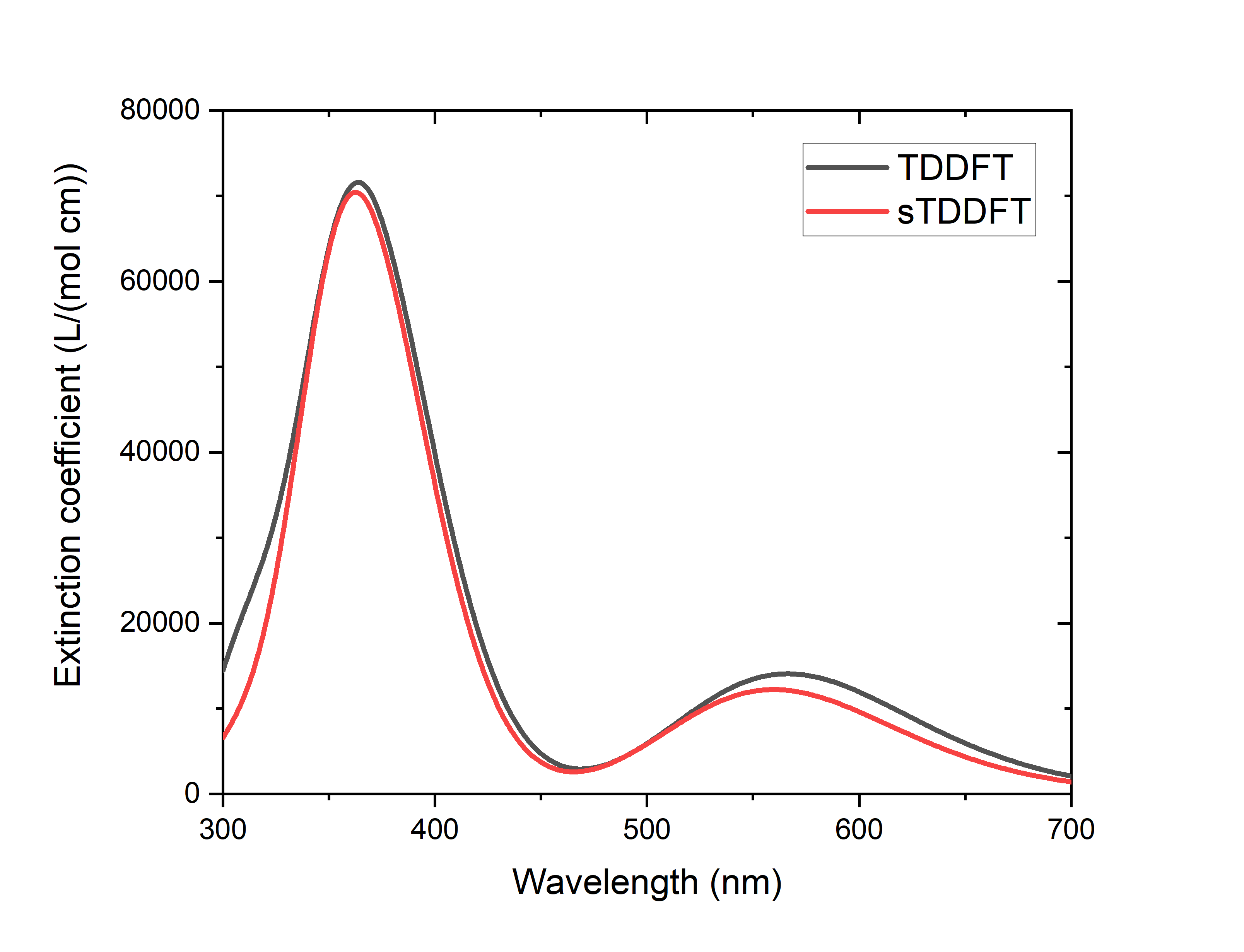
At the same time, sTDDFT saves 95% of the TDDFT calculation time compared with TDDFT (84% of the calculation time if the calculation time of SCF is included), which shows that the acceleration effect is very impressive.
In addition to sTDDFT, the grimmestd keyword can be used for TDA calculations to specify that sTDA calculations are performed, for example:
$tddft
Itda
 1
iwindow
 300 700 nm
grimmestd
$end
Of course, it is also possible to specify the number of excited states calculated instead of the wavelength range:
$tddft
nroot # calculate 100 lowest excited states per irrep
 100
grimmestd
$end
For more information, see Grimmestd Keyword Introduction <grimmestd>.
Restart the TDDFT task that was unexpectedly interrupted
If the TDDFT calculation is terminated unexpectedly, the user may want to reschedule the calculation, that is, when the TDDFT calculation is redone, some intermediate results generated by the previously interrupted TDDFT task are used to reduce or avoid redundant calculation. For details on how to calculate the breakpoint restart of TDDFT, see the corresponding introduction in the FAQ chapter <tddftrestart>.
Mapping of Gaussian broadened absorption spectra
The above calculations only obtain the excitation energy and oscillator intensity of each excited state, and the user often needs to obtain the peak shape of the absorption spectrum predicted theoretically, which requires the absorption of each excited state to be Gaussian broadened according to a certain half-peak width. In BDF, this is achieved via a Python script plotspec.py (located under $BDFHOME/sbin/, where $BDFHOME is the installation path of BDF). After the TDDFT calculation is completed, you need to manually invoke the plotspec.py from the command line. For example, if we have calculated the TDDFT excited state of the C60 molecule with BDF, and the corresponding output file is C60.out, we can run it
$BDFHOME/sbin/plotspec.py C60.out
or
$BDFHOME/sbin/plotspec.py C60
The script outputs the following information on the screen:
==================================
P L O T S P E C
Spectral broadening tool for BDF
==================================
BDF output file: C60.out
1 TDDFT output block(s) found
Block 1: 10 excited state(s)
- Singlet absorption spectrum, spin-allowed
The spectra will be Gaussian-broadened (FWHM = 0.5000 eV) ...
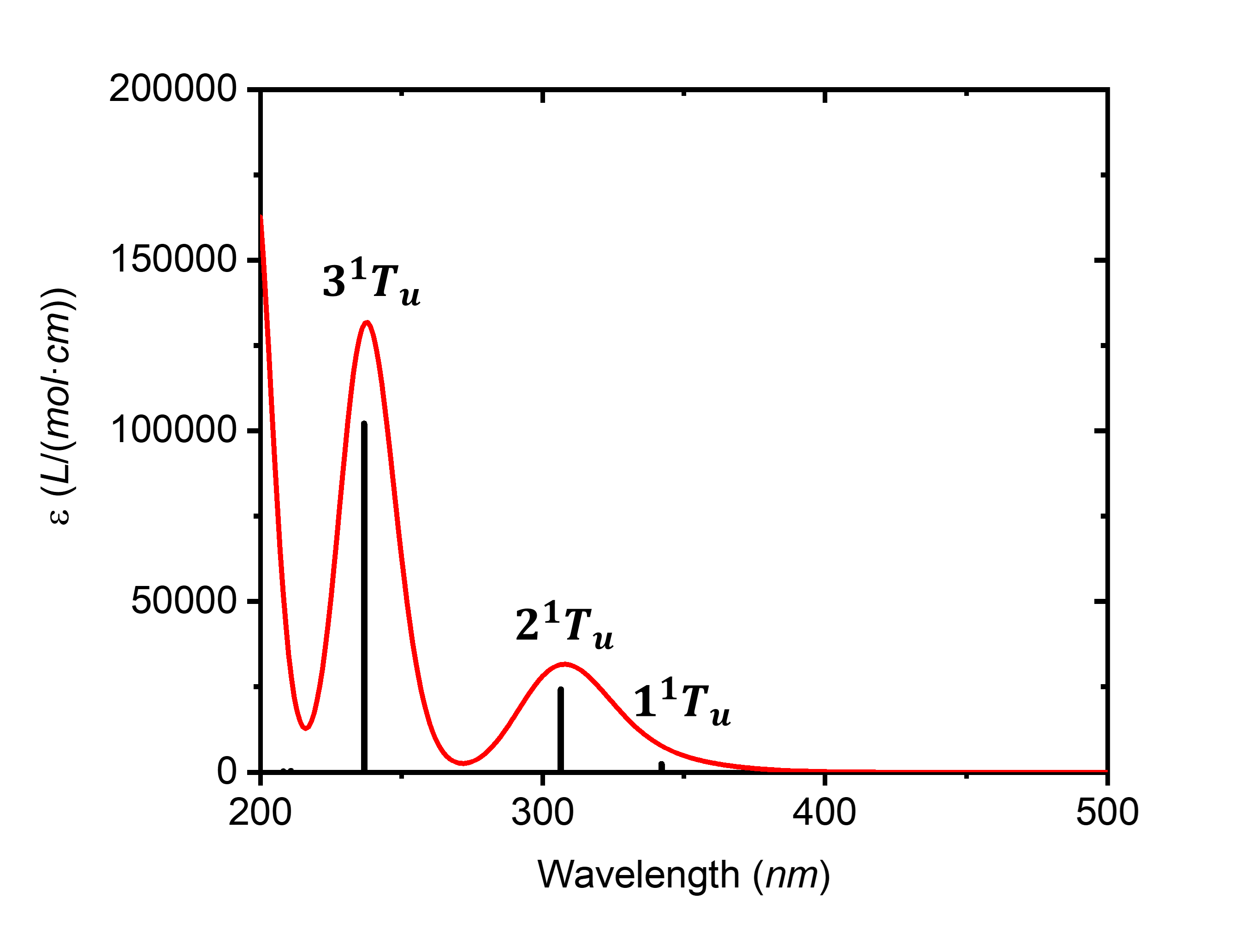
Absorption maxima of spectrum 1 (nm (lg epsilon/(L/(mol cm)))):
- 238 (5.12), 308 (4.50)
plotspec.py: exit successfully
Two files are generated, one is C60.stick.csv, containing the absorption wavelengths and molar extinction coefficients of all excited states, which can be used as a bar plot:
TDDFT Singlets 1,,
Wavelength,Extinction coefficient,
nm,L/(mol cm),
342.867139,2899.779319,
307.302300,31192.802393,
237.635960,131840.430395,
211.765024,295.895849,
209.090150,134.498113,
197.019205,179194.526059,
178.561512,145.257962,
176.943322,54837.570677,
164.778366,548.752301,
160.167663,780.089056,
The other is C60.spec.csv, which contains the absorption spectrum after Gaussian broadening (the default broadening FWHM is 0.5 eV):
TDDFT Singlets 1,,
Wavelength,Extinction coefficient,
nm,L/(mol cm),
200.000000,162720.545118,
201.000000,151036.824457,
202.000000,137429.257570,
...
998.000000,0.000000,
999.000000,0.000000,
1000.000000,0.000000,
These two files can be opened and plotted with Excel, Origin, and other graphing software:
Command line arguments can be used to control the plotting range, Gaussian broadened FWHM, and so on. Example:
# Plot the spectrum in the range 300-600 nm:
 $BDFHOME/sbin/plotspec.py wavelength=300-600nm filename.out

# Plot an X-ray absorption spectrum in the range 200-210 eV,
# using an FWHM of 1 eV:
 $BDFHOME/sbin/plotspec.py energy=200-210eV fwhm=1eV filename.out

# Plot a UV-Vis spectrum in the range 10000 cm-1 to 40000 cm-1,
# where the wavenumber is sampled at an interval of 50 cm-1:
 $BDFHOME/sbin/plotspec.py wavenumber=10000-40000cm-1 interval=50 filename.out

# Plot an emission spectrum in the range 600-1200 nm, as would be
# given by Kasha's rule (i.e. only the first excited state is considered),
# where the wavelength is sampled at an interval of 5 nm:
 $BDFHOME/sbin/plotspec.py -emi wavelength=600-1200nm interval=5 filename.out
If you don’t run $BDFHOME/sbin/plotspec.py without command line arguments, you can list all command line arguments and usages, which will not be repeated here.
Calculation of electron circular dichroism (ECD) spectra
In addition to absorption spectra, BDF also supports the calculation of circular dichroism (ECD) spectra at TDDFT levels. The user only needs to add the ECD keyword to the input of the $tddft module. For example, the following input file calculates the ECD spectrum of (S)-5-methylcyclopenta-2-en-1-one in the range of 160-300 nm at the wB97X/ma-def2-TZVP level with water as solvent:
$COMPASS
Title
 ECD test
Basis
 ma-def2-TZVP
Geometry # B3LYP/def2-SVP geometry
  C   11.03017501307698     -1.06358915357097     18.65132535474617
  C   12.57384005718525     -1.02456284484694     18.65658561738920
  C   12.91529117412091      0.43177145174825     18.82255138315294
  C   11.83078974644673      1.23189442235475     18.82242608164620
  H   10.67388955940226     -1.47007769437446     19.61628109972719
  H   13.00096293117676     -1.40629079282790     17.71067917782706
  H   13.02306939327327     -1.63533989080155     19.45869631125239
  H   13.94838829748073      0.77963695466942     18.91842719115154
  H   11.81586135485978      2.32060314334658     18.90537981712256
  C   10.61010494985639      0.41685642111484     18.65633627754937
  O    9.46516754355473      0.82239910074197     18.54006339565965
  C   10.37591484801120     -1.85714650215417     17.51891751829459
  H   10.61141701850992     -2.93014535161767     17.59810807151853
  H    9.28153845878811     -1.73962079399751     17.55678289237466
  H   10.72376849425688     -1.50217177978463     16.53426564058783
End Geometry
MPEC+COSX
$END

$XUANYUAN
rs
 0.3
$END

$SCF
RKS
DFT
 wB97X
solvent
 water
Solmodel
 SMD # IEFPCM is also a reasonable choice and is almost equally accurate
$END

$tddft
iprt
 3
# To ensure that we get all roots within the window, we use the iVI method.
# Nevertheless, of course, iVI is not mandatory for ECD calculations
idiag
 3# use iVI
iwindow
 160 300 nm
ecd # specifies ECD calculation
solneqlr # linear response solvation, recommended when the number of excited states
         # is large
$end
After the output of the absorption wavelength, oscillator intensity, and transition dipole moment, the transition magnetic dipole moment, and the rotor strength under the length and velocity manifestations are also printed:
*** Ground to excited state Transition magnetic dipole moments (Au) ***
   State          X           Y           Z
      1    -0.001936     0.002882     0.000034
      2    -0.000444    -0.000188    -0.004692
      3    -0.000342    -0.003475    -0.000070
      4    -0.001232     0.000479    -0.001992
      5     0.000581     0.002272    -0.001047
      6    -0.001917     0.003593    -0.000178
      7     0.002065     0.000206    -0.000823


*** Electronic circular dichroism (ECD) rotatory strengths (1e-40 cgs) ***
   State      Length formalism     Velocity formalism
      1               -2.9144               -3.0791
      2               18.0007               17.5760
      3              -25.1038              -25.1132
      4               -7.2316               -7.0551
      5               25.1323               24.4034
      6              -14.9753              -14.2051
      7              -30.6305              -30.8057
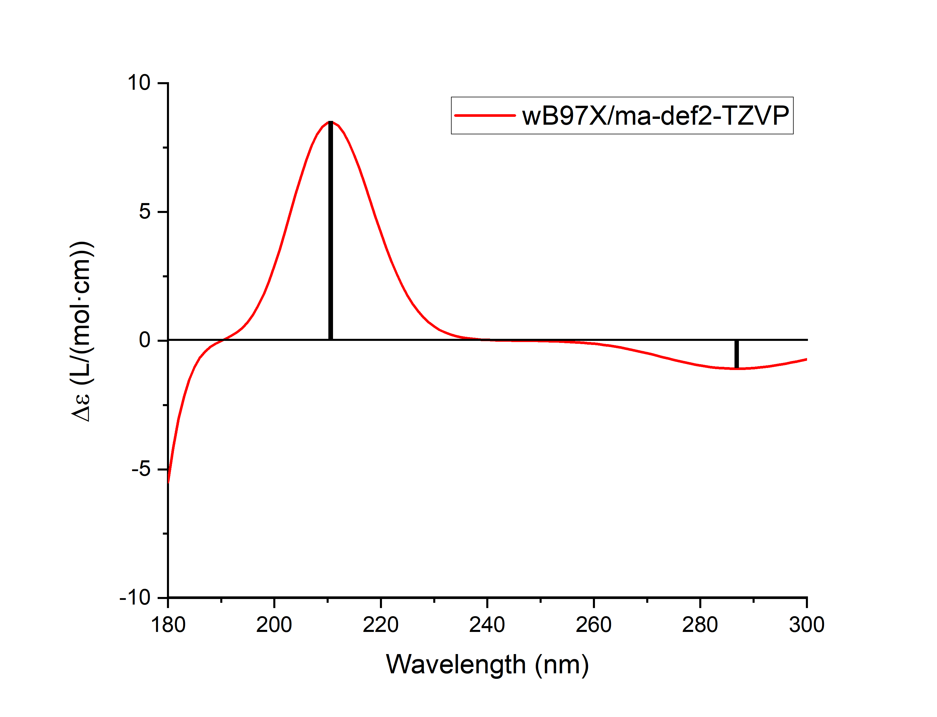
Next, you can use plotspec.py to read the rotor intensity information in the output file, perform Gaussian broadening, and obtain .spec.csv and .stick.csv files to make ECD plots (where the excited states with an absorption wavelength slightly less than 160 nm will have a certain impact on the spectra around 160 nm after Gaussian broadening, and the ECD spectra near 160 nm may not be reliable, so only 180 nm can be used for mapping):
$BDFHOME/sbin/plotspec.py -cd wavelength=180-300 filename.out
Here are the results:
Note
Although the rotor strength under the velocity gauge and the rotor strength under the length gauge are strictly equal when the basis set tends to be complete, when the size of the basis set is limited, the rotor strength under the velocity gauge does not depend on the orientation and center position of the molecule, but the rotor strength under the length gauge is dependent on the orientation and center position of the molecule. Therefore, at least when the molecule is relatively large and the basis set is not too large, the rotor strength results under the velocity gauge are more reliable. plotspec.py by default, the ECD diagram is plotted with the rotor strength under the velocity gauge, if you need to use the rotor strength under the length gauge to plot the ECD diagram, you should change the -cd in the command line argument of the plotspec.py to -cdl.
Due to the difference between BDF and other programs to determine the molecular standard orientation and the origin of molecular coordinates, the rotor strength calculated by BDF under the length representation may be slightly different from other programs, which is a normal phenomenon and is caused by the theoretical defects of the rotor strength under the above length gauge, and does not mean that the calculation results are wrong. However, the rotor strength under the velocity gauge should be in good agreement with other procedures.
For flexible molecules, the ECD calculation results of a single conformation are not reliable, it is recommended to combine CREST, Molclus and other software to perform conformational search, calculate the ECD spectra for all major conformations separately, and then perform Boltzmann weighted average.
Optimization of excited state structure
BDF not only supports the calculation of TDDFT single-point energy (i.e., the excitation energy under a given molecular structure), but also supports the structural optimization and numerical frequency calculation of the excited state. To do this, it is necessary to add the $resp module after the $tddft module to calculate the gradient of TDDFT energy, and the $bdfopt module after the $compass module to use the TDDFT gradient information for structure optimization and frequency calculation (see GeomOptimization<> for details).
The following is an example of optimizing the structure of the first excited state of butadiene at the B3LYP/cc-pVDZ level:
$COMPASS
Title
 C4H6
Basis
 CC-PVDZ
Geometry # Coordinates in Angstrom. The structure has C(2h) symmetry
 C -1.85874726  -0.13257980  0.00000000
 H -1.95342119  -1.19838319  0.00000000
 H -2.73563916   0.48057645  0.00000000
 C -0.63203020   0.44338226  0.00000000
 H -0.53735627   1.50918564  0.00000000
 C  0.63203020  -0.44338226  0.00000000
 H  0.53735627  -1.50918564  0.00000000
 C  1.85874726   0.13257980  0.00000000
 H  1.95342119   1.19838319  0.00000000
 H  2.73563916  -0.48057645  0.00000000
End Geometry
$END

$BDFOPT
solver
 1
$END

$XUANYUAN
$END

$SCF
RKS
dft
 B3lyp
$END

$TDDFT
nroot
# The ordering of irreps of the C(2h) group is: Ag, Au, Bg, Bu
# Thus the following line specifies the calculation of the 1Bu state, which
# happens to be the first excited state for this particular molecule.
 0 0 0 1
istore
 1
# TDDFT gradient requires tighter TDDFT convergence criteria than single-point
# TDDFT calculations, thus we tighten the convergence criteria below.
crit_vec
 1.d-6 # default 1.d-5
crit_e
 1.d-8 # default 1.d-7
$END

$resp
Geom
norder
 1 # first-order nuclear derivative
method
 2 # TDDFT response properties
nfiles
 1 # must be the same number as the number after the istore keyword in $TDDFT
iroot
 1 # calculate the gradient of the first root. Can be omitted here since only
   # one root is calculated in the $TDDFT block
$end
Note that in the above example, the meaning of the keyword ‘’iroot’’ in the ‘’$resp’’ module is different from the keyword ‘’’iroot’’ in the ‘’$tddft’’ module. The former refers to the calculation of the gradient of the first few excited states, while the latter refers to the number of excited states that are calculated in total for each irreducible representation.
After the molecular structure is optimized and converged, the converged structure is output in the main output file:
 Good Job, Geometry Optimization converged in     5 iterations!

Molecular Cartesian Coordinates (X,Y,Z) in Angstrom :
   C          -1.92180514       0.07448476       0.00000000
   H          -2.21141426      -0.98128927       0.00000000
   H          -2.70870517       0.83126705       0.00000000
   C          -0.54269837       0.45145649       0.00000000
   H          -0.31040658       1.52367715       0.00000000
   C           0.54269837      -0.45145649       0.00000000
   H           0.31040658      -1.52367715       0.00000000
   C           1.92180514      -0.07448476       0.00000000
   H           2.21141426       0.98128927       0.00000000
   H           2.70870517      -0.83126705       0.00000000

                    Force-RMS    Force-Max     Step-RMS     Step-Max
 Conv. tolerance :  0.2000E-03   0.3000E-03   0.8000E-03   0.1200E-02
 Current values  :  0.5550E-04   0.1545E-03   0.3473E-03   0.1127E-02
 Geom. converge  :     Yes          Yes          Yes          Yes
In addition, the excitation energy under the excited state equilibrium structure, as well as the total energy and main components of the excited state, can be read from the output of the last TDDFT module of the .out.tmp file:
 Well.     1 w= 5.1695 eV -155.6874121542 a.u.  f= 0.6576 D<Pab>= 0.0000 Ova= 0.8744
      CV(0): Ag( 6 )-> Bu( 10 ) c_i: 0.1224 Per: 1.5% IPA: 17.551 eV Oai: 0.6168
      CV(0): Bg( 1 )-> Au( 2 ) c_i: -0.9479 Per: 89.9% IPA: 4.574 eV Oai: 0.9035

...

  No. Pair   ExSym   ExEnergies  Wavelengths      f     D<S^2>          Dominant Excitations             IPA   Ova     En-E1

    1 Bu 1 Bu 5.1695 eV 239.84 nm 0.6576 0.0000 89.9% CV(0): Bg( 1 )-> Au( 2 ) 4.574 0.874 0.0000
Among them, the wavelength corresponding to the excitation energy under the excited state equilibrium structure (240 nm) is the fluorescence emission wavelength of butadiene.
Note
The optimized excited state structure of some systems will oscillate without convergence, which is generally due to the optimization near the conical intersection. If the optimization is near the conical intersection of the excited state and the ground state, and full TDDFT is used instead of TDA, the structure optimization may even be error-exited due to the excitation energy becoming imaginary or complex. These two situations are normal, and the causes and solutions are detailed in Geometric Optimization Non-Convergent Solution <geomoptnotconverged>.
Spin-orbit coupling calculation based on sf-X2C/TDDFT-SOC
Relativistic effects include scalar relativity and spin-orbit coupling (SOC). Relativistic calculations require the use of a basis set optimized for relativistic effects, and choose the right Hamiltonian**. BDF supports all-electron sf-X2C/TDDFT-SOC calculations, where sf-X2C refers to the consideration of scalar relativistic effects by Hamiltonian of an exact two-component (X2C) without spin, and TDDFT-SOC refers to the calculation of spin-orbit coupling based on TDDFT. Note that although TDDFT is an excited state method, TDDFT-SOC can be used to calculate the contribution of SOC not only to the energy and properties of the excited state, but also to calculate the contribution of SOC to the energy and properties of the ground state.
Taking a molecule with a ground state as a singlet as an example, the sf-X2C/TDDFT-SOC calculation needs to call TDDFT three times in order to complete the calculation. Among them, the first calculation uses R-TDDFT to compute the singlet state, The second time the triplet state was calculated by SF-TDDFT, and wave functions calculated by the first two TDDFT was read in for the last time, and the state interaction (SI) method was used to calculate the spin-orbit couplings for these states. This is clearly seen from the advanced inputs for the sf-X2C/TDDFT-SOC calculation for the :math:’ce{CH2S}’ molecule below.
$COMPASS
Title
 ch2s
Basis # Notice: we use relativistic basis set contracted by DKH2
  cc-pVDZ-DK
Geometry
C       0.000000    0.000000   -1.039839
S       0.000000    0.000000    0.593284
H       0.000000    0.932612   -1.626759
H       0.000000   -0.932612   -1.626759
End geometry
$END

$xuanyuan
heff  # ask for sf-X2C Hamiltonian
 3
hsoc  # set SOC integral as 1e+mf-2e
 2
$end

$scf
RKS
dft
  PBE0
$end

#1st: R-TDDFT, calculate singlets
$tddft
ISF
 0
idiag
 1
iroot
 10
Itda
 0
istore # save TDDFT wave function in the 1st scratch file
 1
$end

#2nd: spin-flip tddft, use close-shell determinant as reference to calculate triplets
$tddft
isf # notice here: ask for spin-flip up calculation
 1
Itda
 0
idiag
 1
iroot
 10
istore # save TDDFT wave function in the 2nd scratch file, must be specified
 2
$end

#3rd: tddft-soc calculation
$tddft
isoc
 2
nprt # print level
 10
nfiles
 2
ifgs # whether to include the ground state in the SOC treatment. 0=no, 1=yes
 1
imatsoc
 8
 0 0 0 2 1 1
 0 0 0 2 2 1
 0 0 0 2 3 1
 0 0 0 2 4 1
 1 1 1 2 1 1
 1 1 1 2 2 1
 1 1 1 2 3 1
 1 1 1 2 4 1
imatrso
 6
 1 1
 1 2
 1 3
 1 4
 1 5
 1 6
idiag # full diagonalization of SO Hamiltonian
 2
$end
Warning
Calculations must be performed in the order of isf=0, isf=1. When the SOC treatment does not consider the ground state (i.e., ‘’ifgs=0’’), the more excited states ‘’iroot’’’ are calculated, the more accurate the result is; When considering the ground state (i.e., ‘’ifgs=1’’’), too much ‘’iroot’’ will reduce the accuracy, which is manifested in the underestimation of the ground state energy.
The keyword imatsoc controls which SOC matrix elements \(<A|hso|B>\) to be printed,
‘’8’’ means that you want to print SOC between 8 sets of spinor states, and 8 lines of integer arrays are entered in the following order;
The input format for each line is fileA symA stateA fileB symB stateB, which represents the matrix elements <fileA,symA,stateA|hsoc|fileB,symB,stateB>, where
fileA symA stateA represents the irreducible root of stateA in file fileA; For example, ‘’1 1 1’’ represents the 1st root of the 1st irreducible representation calculated by the 1st TDDFT;
‘’0 0 0’’ denotes the ground state
Note
The program can only print a maximum of 4000 SOC matrix elements at a time.
The printout of the coupling matrix element is as follows,
  [tddft_soc_matsoc]

Print selected matrix elements of [Hsoc]

SocPairNo. =    1   SOCmat = <  0  0  0 |Hso|  2  1  1 >     Dim =    1    3
  mi/mj ReHso(au) cm^-1 ImHso(au) cm^-1
 0.0 -1.0      0.0000000000      0.0000000000      0.0000000000      0.0000000000
 0.0  0.0      0.0000000000      0.0000000000      0.0000000000      0.0000000000
 0.0  1.0      0.0000000000      0.0000000000      0.0000000000      0.0000000000

SocPairNo. =    2   SOCmat = <  0  0  0 |Hso|  2  2  1 >     Dim =    1    3
  mi/mj ReHso(au) cm^-1 ImHso(au) cm^-1
 0.0 -1.0      0.0000000000      0.0000000000      0.0000000000      0.0000000000
 0.0  0.0      0.0000000000      0.0000000000      0.0007155424    157.0434003237
 0.0  1.0      0.0000000000      0.0000000000     -0.0000000000     -0.0000000000

SocPairNo. =    3   SOCmat = <  0  0  0 |Hso|  2  3  1 >     Dim =    1    3
  mi/mj ReHso(au) cm^-1 ImHso(au) cm^-1
 0.0 -1.0     -0.0003065905    -67.2888361761      0.0000000000      0.0000000000
 0.0  0.0      0.0000000000      0.0000000000     -0.0000000000     -0.0000000000
 0.0  1.0     -0.0003065905    -67.2888361761     -0.0000000000     -0.0000000000
Here, ‘’< 0 0 0 | Hso| 2 2 1 >’’ represents the matrix element ‘’<S0| Hso| T1>’’ , giving the actual part ReHso and the imaginary part ImHso, respectively. Since S0 has only one component, mi is 0. T1 (spin S=1) has 3 components (Ms=-1,0,1), and these 3 components are numbered by mj. where the component of ‘’Ms=0’’ is coupled with the ground state, and the imaginary part of the matrix element is ‘’0.0007155424 au’’.
Warning
When comparing the results of different programs, it is important to note that the so-called spherical tensor is given here, not the cartesian tensor, i.e. T1 is T_{-1}, T_{0}, T_{1}, not Tx, Ty, Tz, and there is a unitary transformation between the two.
The SOC is calculated as follows,
     Totol No. of States:   161  Print:    10

 In.     1 w= -0.0006 eV
      Spin: |Gs,1>    1-th Spatial:  A1;  OmegaSF=      0.0000eV  Cr=  0.0000  Ci=  0.9999  Per:100.0%
    SumPer: 100.0%

 In.     2 w= 1.5481 eV
      Spin: |S+,1>    1-th Spatial:  A2;  OmegaSF=      1.5485eV  Cr=  0.9998  Ci= -0.0000  Per:100.0%
    SumPer: 100.0%

 In.     3 w= 1.5482 eV
      Spin: |S+,3>    1-th Spatial:  A2;  OmegaSF=      1.5485eV  Cr=  0.9998  Ci=  0.0000  Per:100.0%
    SumPer: 100.0%

 In.     4 w= 1.5486 eV
      Spin: |S+,2>    1-th Spatial:  A2;  OmegaSF=      1.5485eV  Cr=  0.9999  Ci=  0.0000  Per:100.0%
    SumPer: 100.0%

 In.     5 w= 2.2106 eV
      Spin: |So,1>    1-th Spatial:  A2;  OmegaSF=      2.2117eV  Cr= -0.9985  Ci=  0.0000  Per: 99.7%
    SumPer:  99.7%

 In.     6 w= 2.5233 eV
      Spin: |S+,1>    1-th Spatial:  A1;  OmegaSF=      2.5232eV  Cr=  0.9998  Ci=  0.0000  Per:100.0%
    SumPer: 100.0%

 In.     7 w= 2.5234 eV
      Spin: |S+,3>    1-th Spatial:  A1;  OmegaSF=      2.5232eV  Cr=  0.9998  Ci= -0.0000  Per:100.0%
    SumPer: 100.0%

 In.     8 w= 2.5240 eV
      Spin: |S+,2>    1-th Spatial:  A1;  OmegaSF=      2.5232eV  Cr=  0.0000  Ci= -0.9985  Per: 99.7%
    SumPer:  99.7%

 In.     9 w= 5.5113 eV
      Spin: |S+,1>    1-th Spatial:  B2;  OmegaSF=      5.5115eV  Cr= -0.7070  Ci= -0.0000  Per: 50.0%
      Spin: |S+,3>    1-th Spatial:  B2;  OmegaSF=      5.5115eV  Cr=  0.7070  Ci=  0.0000  Per: 50.0%
    SumPer: 100.0%

 In.    10 w= 5.5116 eV
      Spin: |S+,1>    1-th Spatial:  B2;  OmegaSF=      5.5115eV  Cr= -0.5011  Ci= -0.0063  Per: 25.1%
      Spin: |S+,2>    1-th Spatial:  B2;  OmegaSF=      5.5115eV  Cr=  0.7055  Ci=  0.0000  Per: 49.8%
      Spin: |S+,3>    1-th Spatial:  B2;  OmegaSF=      5.5115eV  Cr= -0.5011  Ci= -0.0063  Per: 25.1%
    SumPer: 100.0%

*** List of SOC-SI results ***

 No.      ExEnergies Dominant Excitations Esf dE Eex(eV) (cm^-1)

   1      -0.0006 eV   100.0%  Spin: |Gs,1>    0-th   A1    0.0000   -0.0006    0.0000         0.00
   2       1.5481 eV   100.0%  Spin: |S+,1>    1-th   A2    1.5485   -0.0004    1.5487     12491.27
   3       1.5482 eV   100.0%  Spin: |S+,3>    1-th   A2    1.5485   -0.0004    1.5487     12491.38
   4       1.5486 eV   100.0%  Spin: |S+,2>    1-th   A2    1.5485    0.0001    1.5492     12494.98
   5       2.2106 eV    99.7%  Spin: |So,1>    1-th   A2    2.2117   -0.0011    2.2112     17834.44
   6       2.5233 eV   100.0%  Spin: |S+,1>    1-th   A1    2.5232    0.0002    2.5239     20356.82
   7       2.5234 eV   100.0%  Spin: |S+,3>    1-th   A1    2.5232    0.0002    2.5239     20356.99
   8       2.5240 eV    99.7%  Spin: |S+,2>    1-th   A1    2.5232    0.0008    2.5246     20362.08
   9       5.5113 eV    50.0%  Spin: |S+,1>    1-th   B2    5.5115   -0.0002    5.5119     44456.48
  10       5.5116 eV    49.8%  Spin: |S+,2>    1-th   B2    5.5115    0.0001    5.5122     44458.63
The output here has two parts, the first part gives the energy and composition of each SOC-SI state with respect to the S0 state, for example
``No. 10 w= 5.5116 eV’’ means that the energy of the 10th ‘’SOC-SI’’’ state is ‘’5.5116 eV’’, note that here is the energy relative to the S0 state;
The following three lines are the components of this state,
``Spin: | S+,1> 1-th Spatial: B2; ‘’ means that this is the first triplet state with symmetry of B2 (with respect to the S-state spin +1, and therefore S+);
‘’OmegaSF= 5.5115eV’’ is the energy relative to the first spinor state;
‘’Cr= -0.5011 Ci= -0.0063’’ is the real and imaginary part of the wave function of this component in the spinor state, and the percentage is ‘’25.1%’’.
The second part summarizes the results of the SOC-SI states.
ExEnergies lists the excitation energy after considering the SOC. ‘’Esf’’ is the excitation energy when the original SOC is not considered; * The excited state is expressed with ‘’Spin: | S,M> n-th sym’’ to denote spin | Gs, 1>, the spatial symmetry is the nth state of sym. For example, | Gs,1> represents the ground state, | So,1> represents the excited state in which the total spin and ground state are the same, | S+,2> represents the excited state of the total spin plus 1. M is the component of the spin projection (in total 2S+1).
The keyword ‘’imatrso’’ specifies which sets of transition dipole moments between spinor states to be calculated and printed. Here it is specified to print the ‘’6’’ group of transition dipole moments,
‘’1 1’’ denotes the ground state intrinsic dipole moment;
‘’1 2’’ denotes the transition dipole moment between the first and second spinor states.
Note
The program can only print up to 4000 sets of transition dipole moments at a time.
The output of the transition dipole moment is as follows:
[tddft_soc_matrso]: Print selected matrix elements of [dpl]

 No.  ( I , J ) |rij|^2 E_J-E_I fosc rate(s^-1)
-------------------------------------------------------------------------------
  1 1 1 0.472E+00 0.0000000000 0.0000000000 0.000E+00
  Details of transition dipole moment with SOC (in a.u.):
                  <I|X|J>       <I|Y|J>       <I|Z|J>        (also in debye)
         Real= -0.113E-15 -0.828E-18 0.687E+00 -0.0000 -0.0000 1.7471
         Imag=  -0.203E-35     0.948E-35     0.737E-35    -0.0000   0.0000   0.0000
         Norm=   0.113E-15     0.828E-18     0.687E+00


 No.  ( I , J ) |rij|^2 E_J-E_I fosc rate(s^-1)
-------------------------------------------------------------------------------
  2 1 2 0.249E-05 1.548720567 0.000000095 0.985E+01
  Details of transition dipole moment with SOC (in a.u.):
                  <I|X|J>       <I|Y|J>       <I|Z|J>        (also in debye)
         Real= -0.589E-03 0.207E-07 -0.177E-15 -0.0015 0.0000 -0.0000
         Imag=  -0.835E-08     0.147E-02    -0.198E-16    -0.0000   0.0037  -0.0000
         Norm=   0.589E-03     0.147E-02     0.178E-15
Hint
imatsoc is set to -1 to specify that all coupling matrix elements are printed;
By default, the transition dipole moment is not calculated, and the transition dipole moment between all spinor states can be printed by setting imatrso to ‘’-1’’, and the transition dipole moment between all ground spinor states and all excited spinor states can be printed by setting imatrso to ‘’-2’’.
The reference state of the SOC calculation must be either RHF/RKS or ROHF/ROKS, UHF/UKS is not supported.
When the reference state of the SOC calculation is ROHF/ROKS, the TDDFT calculation of isf=0 must use X-TDA (i.e., itest=1, icorrect=1, isf=0, itda=1; full X-TDDFT is not supported), and the TDDFT calculation of isf=1 must use SF-TDA (i.e., isf=1, itda=1; full SF-TDDFT is not supported).
TDDFT-SOC spin-orbit coupling calculation using ECP base set
In addition to the sf-X2C all-electron scalar relativistic Hamiltonian, the pseudopotential can also be used for TDDFT-SOC spin-orbit coupling calculations, in which the spin-orbit coupling pseudopotential (SOECP) is the first choice. To do this, you need to select the appropriate spin-orbit-coupled Pseudopotential Basis Set <soecp-bas> and set the hsoc to 10 in the Xuanyuan module (you can also write other values, But it will be treated as 10). Other inputs are similar or identical to the sf-X2C/TDDFT-SOC inputs (e.g. core electrons are excluded when specifying orbital occupancy in ‘’scf’’).
In the example below, the closed-shell ground state of the InBr molecule is calculated under the symmetry of the :math:’C_{2v}’ point group, and the lowest three excited states of the InBr molecule :math:’^3Pi’ (B1+B2), :math:’^1Pi’ (B1+B2), :math:’^3Sigma^+’ (A1), where the first two Λ-S states are bound states that have been extensively experimentally studied, THE LAST TWO Λ-S STATES ARE REPULSIVE STATES AND ARE NOT MUCH OF AN EXPERIMENTAL CONCERN. In the input, the energy of the Λ-S state is calculated and the wave function is stored at the TDDFT level (Tamm-Dancoff approximation is used here), and then the energy of the Ω state after spin-orbit coupling is calculated.
$COMPASS
Title
 soecp test: InBr
Basis-block
  cc-pVTZ-PP
end basis
Geometry
  In  0.0  0.0  0.0
  Br  0.0  0.0  2.45
END geometry
group
 C(2v)      # Abelian symmetry must be used for SOC
$END

$XUANYUAN
 hsoc
  10
$END

$scf
  rks
  dft
   pbe0
$end

$TDDFT
ISF
 0
ITDA
 1
istore
 1
# 1Pi state: A1, A2, B1, B2
nroot
  0 0 1 1
$END

$TDDFT
ISF
 1
ITDA
 1
istore
 2
# 3Sigma+ and 3Pi states: A1, A2, B1, B2
nroot
  1 0 1 1
$END

$TDDFT
isoc
 2
nfiles
 2
ifgs
 1
idiag
 2
$END
The calculated output of SOECP/TDFT-SOC is similar to that of the sf-X2C/TDDFT-SOC. The results are summarized below and compared to those of the two-component EOM-CCSD.
In addition to the SOECP basis set, the above calculation can also be done with a scalar ECP basis set combined with the effective nuclear charge approximation (Zeff) <so1e-zeff>’. As a test, first remove the SO pseudopotential part of the Br basis set and redo the above calculation, but you will find that the results are poor: The split between :math:’^3Pi_2’ and :math:’^3Pi_1’ is only 850 cm :math:’^{-1}’, while the split between :math:’^3Sigma^+’ is almost zero. This is because the ECP base set of Br with 10 cores does not have a specially optimized effective nuclear charge, and the program can only take the actual number of nuclear charges 35:
SO-1e[BP]
          Zeff for Wso
----------------------------------
 IAtm     ZA    NCore         Zeff
----------------------------------
    1     49       28        SOECP
    2 35 10 N.A.
----------------------------------
For Br in the above example, you may wish to use the scalar ECP base set cc-pVTZ-ccECP with 28 core electrons instead, and the input part of the basis set is modified as follows:
Basis-block
  cc-pvtz-pp
  Br=cc-pvtz-ccecp
end basis
Track occupancy is not specified in modules after xuanyuan, so there is no need to modify the input. It can be seen at the beginning of the TDDFT-SOC calculation output
SO-1e[BP]
          Zeff for Wso
----------------------------------
 IAtm     ZA    NCore         Zeff
----------------------------------
    1     49       28        SOECP
    2     35       28     1435.000
----------------------------------
This shows that in the single-electron spin-orbit integral of Br, the default nuclear charge number 35 is replaced with an optimized 1435.000 (in general, the larger the ECP core electron number NCore, the larger the effective nuclear charge Zeff), SOECP integrals are still calculated for the In atom. The results are as follows, and it can be seen that the SOC splitting has been significantly improved:
Finally, TDDFT-SOC calculations can also be combined with SOECP (or scalar ECP) basis sets with all-electron non-relativistic basis sets. The BDF program has optimized Zeff for the all-electron non-relativistic basis set of the main group elements prior to Xe (except for the heavier noble gas elements). For example, if you continue to use cc-pVTZ-PP for In, and cc-pVTZ for Br, you will get similar results to SOECP/TDDFT-SOC. Detailed results omitted.
Attention
Precautions when using the effective nuclear charge method for TDDFT-SOC calculations: Optimized effective nuclear charge <SO1e-zeff>’ must be used to ensure accuracy. To do this, check the Zeff value printed in the output file and try not to show N.A., which is especially important for the ECP baseset.
Notes on all-electron basis sets when combining SOECP or scalar ECP with all-electron basis groups: Since atoms using all-electron basis sets do not consider scalar relativistic correspondence, they cannot be heavy atoms, and non-relativistic basis sets must be used.
Calculation of the first-order non-adiabatic coupled matrix element (fo-NACME).
As mentioned earlier, (first-order) non-adiabatic coupling matrix elements are of great significance in the non-radiative transition process, and one of their main uses is to calculate the internal convension rate constant (see azulene-example> for calculating the internal convension rate constant with BDF-MOMAP< ). In BDF, there are some differences in how the NACME input files between the ground state and the excited state, and between the excited state and the excited state are written separately.
Note
NACME between ground state and excited state, and NACME between excited state and excited state support R-TDDFT and U-TDDFT, but X-TDDFT is not supported.
NACME between ground state and excited state: :math:’ce{NO3}’ radical D0/D1 NACME (GB3LYP/cc-pVDZ)
$COMPASS
Title
 NO3 radical NAC, 1st excited state
Basis
 cc-pvdz
Geometry
N 0.00000000000 0.0000000000 -0.1945736441
O             -2.0700698389         0.0000000000        -1.1615808530
O              2.0700698389        -0.0000000000        -1.1615808530
O             -0.0000000000         0.0000000000         2.4934136445
End geometry
unit
 bohr
$END

$XUANYUAN
$END

$SCF
DOOR
dft
 GB3LYP
spinmulti
 2
$END

$tddft
iroot
 1 # One root for each irrep
istore
 1 # File number, to be used later in $resp
crit_vec
 1.d-6
crit_e
 1.d-8
gridtol
 1.d-7 # tighten the tolerance value of XC grid generation. This helps to
       # reduce numerical error, and is recommended for open-shell molecules
$end

$resp
iprt
 1
QUAD # quadratic response
FNAC # first-order NACME
single # calculation of properties from single residues (ground state-excited
       # state fo-NACMEs belong to this kind of properties)
norder
 1
method
 2
nfiles
 1 # must be the same as the istore value in the $TDDFT block
states
 1 # Number of excited states for which NAC is requested.
# First number 1: read TDDFT results from file No. 1
# Second number 2: the second irrep, in this case A2
#   (note: this is the pair symmetry of the particle-hole pair, not
#   the excited state symmetry. One must bear this in mind because the
#   ground state of radicals frequently does not belong to the totally
#   symmetric irrep)
#   If no symmetry is used, simply use 1.
# Third number 1: the 1st excited state that belongs to this irrep
 1 2 1
$end
Note: The irreducible representation specified in the $resp module is a pair irrep (i.e., the direct product of the irreducible representation of the occupied and empty orbits involved in the transition; For abelian point groups, pair irrep can be obtained from the direct product of the irreducible representation of the ground state and the irreducible representation of the excited state), but not the irrep of the excited state. The ground state (D0) of the molecule belongs to the B1 irreducible representation, and the first binary excited state (D1) belongs to the B2 irreducible representation, so the pair irrep of the D1 state is the direct product of B1 and B2, i.e., A2. Pair irrep can also be read from the output of the TDDFT module, i.e. in the Pair column of the following output sections:
No. Pair   ExSym   ExEnergies  Wavelengths      f     D<S^2>          Dominant Excitations             IPA   Ova     En-E1

  1 A2 1 B2 0.8005 eV 1548.84 nm 0.0000 0.0186 98.2% CO(bb): B2( 2 )-> B1( 5 ) 3.992 0.622 0.0000
  2 B1 1 A1 1.9700 eV 629.35 nm 0.0011 0.0399 92.2% CO(bb): A1(8)-> B1(5) 3.958 0.667 1.1695
  3 B2 1 A2 2.5146 eV 493.06 nm 0.0000 0.0384 98.4% CO(bb): A2(1)-> B1(5) 4.159 0.319 1.7141
  4 A1 2 B1 2.6054 eV 475.87 nm 0.0171 0.0154 87.7% CO(bb): B1( 4 )-> B1( 5 ) 3.984 0.746 1.8049
After the calculation is completed, at the end of the output section of the $resp module, you can see the result of the NACME calculation:
Gradient contribution from Final-NAC(R)-Escaled
   1        0.0000000000       -0.0000000000        0.0000000000
   2       -0.0000000000       -0.1902838724        0.0000000000
   3       -0.0000000000        0.1902838724        0.0000000000
   4       -0.0000000000        0.0000000000        0.0000000000
It can be found that the calculation results have N rows (where N is the number of atoms of the system), and each row has 3 real numbers, representing the x, y, and z components of the NACME of the atoms. Note that this result does not include the contribution of the electron translation factor (ETF), and for some molecules, NACME excluding ETF may not have translational invariance, which may lead to errors in subsequent calculations such as kinetic simulations. In this case, you need to use NACME with ETF in mind, which can be read later in the output file:
Gradient contribution from Final-NAC(S)-Escaled
   1        0.0000000000       -0.0000000000        0.0000000000
   2       -0.0000000000       -0.1920053581        0.0000000000
   3       -0.0000000000        0.1920053581        0.0000000000
   4       -0.0000000000        0.0000000000       -0.0000000000
The program also outputs vectors named dpq-R, Final-NAC(R), dpq-S, Final-NAC(S), etc., which are intermediate variables and are only used to monitor the calculation process, not the final NACME, and can be ignored by the user in general.
NACME between excited and excited states: T1/T2 NACME (BH&HLYP/def2-SVP) of acetophenone
$compass
title
 PhCOMe
basis
 def2-SVP
geometry
        C             -0.3657620861         4.8928163606         0.0000770328
        C             -2.4915224786         3.3493223987        -0.0001063823
        C             -2.2618953860         0.7463412225        -0.0001958732
        C              0.1436118499        -0.3999193588        -0.0000964543
        C              2.2879147462         1.1871091769         0.0000824391
        C              2.0183382809         3.7824607425         0.0001740921
        H -0.5627800515 6.9313968857 0.0001389666
        H -4.3630645857 4.1868310874 -0.0002094148
        H -3.9523568496 -0.4075513123 -0.0003833263
        H 4.1604797959 0.3598389310 0.0001836001
        H 3.6948496439 4.9629708946 0.0003304312
        C              0.3897478526        -3.0915327760        -0.0002927344
        O              2.5733215239        -4.1533492423        -0.0002053903
        C             -1.8017552120        -4.9131221777         0.0003595831
        H -2.9771560760 -4.6352720097 1.6803279168
        H -2.9780678476 -4.6353463569 -1.6789597597
        H -1.1205416224 -6.8569277129 0.0002044899
end geometry
unit
 bohr
nosymm
$end

$XUANYUAN
$END

$SCF
rks
dft
 bhhlyp
$END

$tddft
isf # request for triplets (spin flip up)
 1
ialda # use collinear kernel (NAC only supports collinear kernel)
 4
iroot
 2 # calculate T1 and T2 states
crit_vec
 1.d-6
crit_e
 1.d-8
istore
 1
iprt
 2
$end

$resp
iprt
 1
QUAD
FNAC
double # calculation of properties from double residues (excited state-excited
       # state fo-NACMEs belong to this kind of properties)
norder
 1
method
 2
nfiles
 1
pairs
 1 # Number of pairs of excited states for which NAC is requested.
 1 1 1 1 1 2
noresp # do not include the quadratic response contributions (recommended)
$end
The NACME of T1 and T2 states is calculated:
Gradient contribution from Final-NAC(R)-Escaled
   1        0.0005655253        0.0005095355       -0.2407937116
   2       -0.0006501682       -0.0005568029        0.5339003311
   3        0.0009640605        0.0003767996       -2.6530192038
   4       -0.0013429266       -0.0034063171        1.6760344312
   5        0.0010446538        0.0006384285       -0.8024123329
   6       -0.0001081722       -0.0006245719       -0.0487310115
   7       -0.0000001499        0.0000176176       -0.0730900968
   8       -0.0000214634        0.0000165092        0.3841606239
   9        0.0000026057       -0.0000025322       -0.2553378323
  10       -0.0002028358       -0.0000591642        0.5800987974
  11       -0.0000166820        0.0000105734        0.2713836450
  12       -0.0023404123        0.0052038311        3.5121827769
  13        0.0021749503       -0.0012164868       -2.7480141157
  14        0.0000433873       -0.0011202812        0.2896243729
  15        0.1407516324        0.1432264573       -0.1655701318
  16       -0.1407399684       -0.1429881941       -0.1657943551
  17       -0.0000034197        0.0004577563       -0.0833951446
Localization of excited states
$COMPASS
Basis
 cc-pvdz
Geometry
  C      0.000000    0.000000  0.000000
  C      1.332000    0.000000  0.000000
  H     -0.574301   -0.928785  0.000000
  H     -0.574301    0.928785  0.000000
  H      1.906301    0.928785  0.000000
  H      1.906301   -0.928785  0.000000
  C     -0.000000    0.000000  3.500000
  C      1.332000   -0.000000  3.500000
  H     -0.574301    0.928785  3.500000
  H     -0.574301   -0.928785  3.500000
  H      1.906301   -0.928785  3.500000
  H      1.906301    0.928785  3.500000
End geometry
Group
 C(1)
Nfragment # must input: number of fragment, should be 1
 1
$END

$xuanyuan
$end

$scf
rks
dft
 B3lyp
$end

$TDDFT
ITDA
 1
IDIAG
 1
istore
 1
iroot
  4
crit_e # set a small threshhold for TDDFT energy convergence
  1.d-8
$END

# calculate local excited states (LOCALES)
$elecoup
Local
  1
$END

&database
fragment 1  12 # first fragment with 12 atoms, next line gives the atom list
 1 2 3 4 5 6 7 8 9 10 11 12
&end
TDA calculates 4 excited states and the output is as follows,
No. Pair   ExSym   ExEnergies  Wavelengths      f     D<S^2>          Dominant Excitations             IPA   Ova     En-E1

 1   A    2   A    7.4870 eV    165.60 nm   0.0000   0.0000  82.6%  CV(0):   A(  16 )->   A(  17 )  13.476 0.820    0.0000
 2   A    3   A    8.6807 eV    142.83 nm   0.0673   0.0000  79.6%  CV(0):   A(  16 )->   A(  18 )  14.553 0.375    1.1937
 3   A    4   A    9.0292 eV    137.31 nm   0.0000   0.0000  62.4%  CV(0):   A(  16 )->   A(  20 )  15.353 0.398    1.5422
 4   A    5   A    9.0663 eV    136.75 nm   0.0000   0.0000  50.4%  CV(0):   A(  15 )->   A(  18 )  15.688 0.390    1.5793
The process of localization of the excited states is as follows,
  No.  8 iteration
Pair States :    1   2
aij,bij,abij -.25659893E-01 -.48045653E-11 0.25659893E-01
cos4a,sin4a 0.10000000E+01 -.18724027E-09
cosa,sina 0.10000000E+01 0.00000000E+00
Pair States :    1   3
aij,bee,aby -.40325646E-02 0.35638586E-11 0.40325646E-02
cos4a,sin4a 0.10000000E+01 0.88376974E-09
cosa,sina 0.10000000E+01 0.00000000E+00
Pair States :    1   4
aij,bij,abij -.25679319E-01 -.28753641E-08 0.25679319E-01
cos4a,sin4a 0.10000000E+01 -.11197197E-06
cosa,sina 0.10000000E+01 0.27877520E-07
Pair States :    2   3
aij,bij,abij -.39851115E-02 -.27118892E-05 0.39851124E-02
cos4a,sin4a 0.99999977E+00 -.68050506E-03
cosa,sina 0.99999999E+00 0.17012628E-03
Pair States :    2   4
aij,bij,abij -.42686102E-02 -.95914926E-06 0.42686103E-02
cos4a,sin4a 0.99999997E+00 -.22469825E-03
cosa,sina 0.10000000E+01 0.56174562E-04
Pair States :    3   4
aij,bij,abij -.67873307E-01 -.47952471E-02 0.68042488E-01
cos4a,sin4a 0.99751360E+00 -.70474305E-01
cosa,sina 0.99984454E+00 0.17632279E-01
Sum= 0.13608498 Max Delta= 0.00531009

  No.  9 iteration
Pair States :    1   2
aij,bee,aby -.40325638E-02 0.35621782E-11 0.40325638E-02
cos4a,sin4a 0.10000000E+01 0.88335323E-09
cosa,sina 0.10000000E+01 0.00000000E+00
Pair States :    1   3
aij,bee,aby -.25690755E-01 -.11200070E-08 0.25690755E-01
cos4a,sin4a 0.10000000E+01 -.43595721E-07
cosa,sina 0.10000000E+01 0.10536712E-07
Pair States :    1   4
aij,bee,aby -.25690755E-01 -.10900573E-11 0.25690755E-01
cos4a,sin4a 0.10000000E+01 -.42429944E-10
cosa,sina 0.10000000E+01 0.00000000E+00
Pair States :    2   3
aij,bij,abij -.41480079E-02 -.83549288E-06 0.41480080E-02
cos4a,sin4a 0.99999998E+00 -.20142027E-03
cosa,sina 0.10000000E+01 0.50355067E-04
Pair States :    2   4
aij,bee,aby -.41480100E-02 0.17462423E-06 0.41480100E-02
cos4a,sin4a 0.10000000E+01 0.42098314E-04
cosa,sina 0.10000000E+01 0.10524580E-04
Pair States :    3   4
aij,bij,abij -.68042492E-01 0.19389042E-08 0.68042492E-01
cos4a,sin4a 0.10000000E+01 0.28495490E-07
cosa,sina 0.10000000E+01 0.74505806E-08
Sum= 0.13608498 Max Delta= 0.00000000

***************** Diabatic Hamiltonian matrix ****************
              State1      State2      State3     State4
   State1    7.486977    0.000000    0.000000    0.000000
   State2    0.000000    9.029214   -0.000020    0.000021
   State3    0.000000   -0.000020    8.873501    0.192803
   State4    0.000000    0.000021    0.192803    8.873501**************************************************************
where the diagonal element is the energy of the localized excited state, and the non-diagonal element is the coupling between the two localized states, where the unit of energy is ‘’eV’’.