Application examples
Mössbauer Spectroscopy
In 1958, R. L. Mössbauer discovered the Mössbauer effect while studying γ-ray resonance absorption phenomena. The isomer shift (δᴵˢ) is one of the important observable parameters in Mössbauer spectroscopy, originating from the Coulomb interaction between atomic nuclei of finite size and the surrounding electron distribution. When atoms are in different external environments, the Coulomb energy near the nucleus changes, and δᴵˢ is extremely sensitive to this change, making it useful for studying atomic oxidation states, spin states, and coordination environments. Another important observable parameter is the nuclear quadrupole splitting (ΔE_Q), which arises from the interaction between the electric quadrupole moment (eQ; where e is the proton charge and Q is the nuclear quadrupole moment, NQM) of nuclei with spin quantum number I > 1/2 and the electric field gradient (EFG) around the nucleus. Additionally, when atoms are placed in an external magnetic field, Mössbauer spectra undergo further Zeeman splitting due to the nuclear magnetic moment.
δᴵˢ can be expressed as a linear function of the change in “effective contact density” (ED) or “contact density” (CD) between the test system A and the reference system R:
These two formulas are called calibration equations, where δᴵˢ is the experimental isomer shift of test system A relative to reference system R. The ED or CD values ρ_A and ρ_R can be obtained through theoretical calculations. α and β are parameters to be fitted, with α also known as the nuclear calibration constant. C is an arbitrary constant, usually taken as the integer part of ED or CD. Considering potential errors in the theoretical value of ρ_R, the latter formula is generally used for fitting.
Note
CD assumes a uniform distribution of electron density near the nucleus and thus uses the density at a single point (usually the nuclear center, though some programs use weighted averages of multiple points). ED considers the non-uniform distribution of electron density and is theoretically more reasonable. Many programs calculate CD, while BDF calculates ED. The two are approximately convertible (see Tables S2 and S3 in reference [89]), and the conversion factor can be absorbed into α.
To accurately calculate ED and its relative changes, two factors must be considered:
Atomic nuclei have finite size distributions, and the default point-charge approximation may lead to errors of several orders of magnitude! Set
nuclear=1in thexuanyuanmodule to address this.Relativistic effects must be considered. This is obvious for heavy elements, but even for some light elements it’s essential. Non-relativistic p electrons have no distribution near the nucleus (see Table S6 in reference [89]), leading to qualitatively wrong ED for p-block elements. In BDF, scalar relativistic effects can be included using the sf-X2C Hamiltonian or its local variants, specified via
heff=21(standard sf-X2C),22(sf-X2C-AXR), or23(sf-X2C-AU) in thexuanyuanmodule.
Effective Contact Density of Iron ( \(\ce{^{57}Fe}\) ) Compounds
The probability of γ-ray absorption and emission is proportional to \(\exp(-E_\gamma^2)\). When nuclear excitation energy E_γ exceeds 200 keV, Mössbauer spectroscopy becomes difficult to observe, limiting its application to only a few isotopes. \(\ce{^{57}Fe}\) is one such suitable isotope, though theoretical calculations generally don’t distinguish between isotopes.
Calculating ED requires extremely steep s-type Gaussian basis functions to accurately describe electron distribution near the iron nucleus. For p-block elements with p valence electrons, very steep p-type Gaussian basis functions are also needed, which standard contracted basis sets typically lack. We recommend using all-electron relativistic basis sets like cc-pVnZ or ANO, with their s functions (and p functions for p-block elements) uncontracted. In the following all-electron relativistic calculations, iron uses the ANO-R2 basis set (triple-ζ accuracy) with s functions uncontracted (remove contraction coefficients and set contraction degree to 0), saved under a different name (e.g., ANO-R2-ED). Since iron has no 4*p* valence electrons, p functions don’t need modification. Copy ANO-R2-ED to the $BDF_WORKDIR directory for subsequent calculations (download link: ano-r2-ed.zip). Note: For non-standard basis sets, all letters in the basis set name must be uppercase.
We perform relativistic density functional theory calculations for a series of iron model compounds using the PBE0 functional and sf-X2C-AU relativistic Hamiltonian. Light elements other than iron use the def2-TZVPP basis set, which is all-electron for elements before Kr and suitable for relativistic calculations of the first 18 elements. Spin multiplicities and molecular coordinates are from reference [90]. For \(\ce{FeF6^{4-}}\), the input is:
$compass
 title
   FeF_6^4-
 basis-block
   def2-tzvpp
   Fe = ANO-R2-ED
 end basis
 geometry  # Cartesian coordinates in Ångstroms
   Fe -0.000035  0.000012  0.000014
   F   2.116808 -0.003546  0.032360
   F  -2.116824  0.001611 -0.030945
   F  -0.003602  2.164955  0.001902
   F   0.001648 -2.165219 -0.003295
   F   0.032586  0.003638  2.109790
   F  -0.030580 -0.001452 -2.109825
 end geometry
 MPEC+cosx        # Use MPEC+COSX acceleration
$end

$xuanyuan
 heff      # sf-X2C-AU; must choose 21-23 for ED
   23
 nuclear   # Gaussian finite nucleus model; must set to 1 for ED
   1
$end

$scf
 charge
   -4
 spinmulti
   5
 uks
 dft functional
   pbe0
 grid             # Precision grid required for ED calculation
   ultra fine
 reled
   26             # Calculate ED only for Fe (integers 10-26 equivalent here)
$end
After calculation, ED results appear after SCF population analysis:
Relativistic effective contact densities for the atoms with Za > 25
----------------------------------------------------------------
      No.     Iatm       Za       RMS (fm)            Rho (a.u.)
----------------------------------------------------------------
        1        1       26        3.76842           14552.65555
----------------------------------------------------------------
Following this example, complete ED calculations for other iron compound molecules (input file download: ed-fe.zip). ED results and experimental δᴵˢ values [90] are listed below:
Fitting this data yields the calibration equation:
The significant fitting error may stem from: 1. Small sample size 2. Mössbauer spectra are measured for solid-state systems, inconsistent with gaseous ion models. Cluster models, solvation models [91], or embedding models [92] may be more appropriate. 3. Strong correlation in some iron compounds requires testing other functionals or methods suitable for strongly correlated systems.
Using this calibration equation, we can predict δᴵˢ for iron systems. For example, staggered ferrocene [93] yields ED = 14554.25 a.u. through DFT, giving δᴵˢ = 0.37 mm/s, close to the experimental value of 0.53 mm/s [93].
Notes for Calculating Effective Contact Density in Heavy-Element Compounds
For elements beyond 4d, default Gaussian exponents are insufficient to describe electron distribution near the nucleus. Additional steeper exponents are needed. For example, select the steepest 4-6 s-type Gaussian exponents α from standard cc-pVnZ or ANO basis sets (also consider p-type for p-block heavy elements). These approximately satisfy:
Linear fitting yields parameters A and B. Extrapolation (using intervals of -0.5 or -1 for i) provides steeper Gaussian exponents. Adding 2-5 steeper s functions and 1-3 steeper p functions is usually sufficient, but avoid exponents > 10¹¹ to prevent numerical instability.
EFG Calculation for Iron ( \(\ce{^{57}Fe}\) ) Compounds
EFG calculations have similar relativistic Hamiltonian requirements as ED calculations but different basis set requirements:
Only s electrons and a few p electrons have non-zero distribution near the nucleus, so ED calculations only need modified s and p basis functions.
Nuclear deformation quadrupole moments only interact with EFG from electrons with orbital angular momentum L > 0, so s basis functions don’t need modification. Uncontract p functions (remove contraction coefficients and set contraction degree to 0), and add 1-2 steep p-type Gaussian functions. For transition elements with d valence orbitals (lanthanides/actinides also have f), uncontract d (and f) functions. Since d and f orbitals are farther from the nucleus, steeper d/f functions aren’t needed.
When calculating both ED and EFG, basis function modifications must satisfy both requirements.
The keyword for EFG calculation is relefg. For example, to calculate both ED and EFG, modify the SCF module input as:
$scf
 charge
   -4
 spinmulti
   5
 uks
 dft functional
   pbe0
 grid             # Precision grid required for EFG
   ultra fine
 relefg
   26             # Calculate EFG tensor only for Fe
 reled
   26             # Calculate ED only for Fe
$end
After calculation, EFG tensor results appear after SCF population analysis and ED results:
Relativistic electric field gradients for the atoms with Za > 25
-----------------------------------------------------------------------------
      No.     Iatm       Za       RMS (fm)            EFG tensor (a.u.)
-----------------------------------------------------------------------------
        1        1       26        3.76842      -0.1061    -0.0023     0.1850
                                                -0.0023     0.0395    -0.0018
                                                 0.1850    -0.0018     0.0666

                                     eta           Vaa        Vbb        Vcc
                                   0.64736       0.0395     0.1844    -0.2239

                 NQCC =         -8.4172 MHz with Q(ISO-057) =    160.00 mbarn

-----------------------------------------------------------------------------
Among the 9 components of the EFG tensor, the 6 off-diagonal elements are symmetric. The sum of the 3 diagonal elements is zero. In a special coordinate system \(\{\vec{a},\vec{b},\vec{c}\}\) (principal axes/eigenvectors of the EFG tensor), off-diagonal elements vanish, and diagonal elements (eigenvalues) satisfy \(|V_{aa}| \le |V_{bb}| \le |V_{cc}|\). The EFG tensor can then be described by two parameters: principal value \(V_{cc}\) and asymmetry parameter \(\eta = |(V_{aa} − V_{bb})/V_{cc}|\) (0 ≤ η ≤ 1). When η = 0, the EFG tensor is axially symmetric. Here, η = 0.64736 and \(V_{cc}\) = -0.2239 a.u.
Attention
For molecules in non-Abelian degenerate states, \(V_{cc}\) and η from a single branch are generally meaningless. Calculate EFG tensors for all degenerate branches (by specifying occupations in SCF), average them, then compute \(V_{cc}\) and η.
For isolated atoms, \(V_{aa} = V_{bb} = V_{cc} = 0\). For linear molecules (including diatomic), \(V_{cc} = V_{zz}\) (z-axis along molecular axis). BDF can correct EFG results for open-shell atoms and linear molecules in degenerate states using this property.
The interaction between nuclear quadrupole moment and EFG is typically measured by the nuclear quadrupole coupling constant (NQCC, \(eQq\)), defined as:
where \(V_{cc}\) is in atomic units, nuclear quadrupole moment Q is in Barn (1 Barn = 1.0e-28 m²), and \(eQq\) is in MHz. When the experimental Q value is known, the program prints \(eQq\), here -8.4172 MHz.
The nuclear quadrupole splitting ΔE_Q measured by Mössbauer spectroscopy relates to NQCC. For \(\ce{^{57}Fe}\) I=1/2 → I=3/2 nuclear excitation transition (γ-ray energy 14.412497 KeV ≈ 34.85e11 MHz):
with unit conversion factor 1 mm/s = 11.6248 MHz. Theoretical ΔE_Q can be directly compared with experimental Mössbauer values and combined with ED results to verify iron oxidation state assignments.
Theoretical Insight into the Thermally Activated Delayed Fluorescence (TADF) Mechanism of DPO-TXO2
Thermally Activated Delayed Fluorescence (TADF) materials represent the third generation of pure organic delayed fluorescence materials, developed after fluorescent materials and noble metal phosphorescent materials. Their hallmark features include a small singlet-triplet energy gap (ΔES-T) and positive temperature dependence.
In 2012, the Chiahaya Adachi group at Kyushu University first reported the 4CzIPN molecule with an external quantum efficiency (EQE) exceeding 20% [ ]. This material exhibited an almost negligible energy difference between singlet and triplet states, enabling complete exciton return from the triplet to singlet state under room temperature thermal disturbance (298 K) to emit fluorescence—thus named TADF (Thermally Activated Delayed Fluorescence).
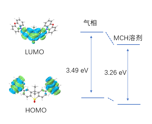
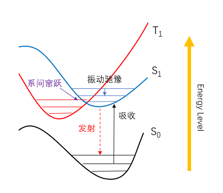
When both S1 and T1 excitations exhibit HOMO→LUMO characteristics, their energy difference equals 2*K, where K is the exchange integral between HOMO and LUMO. As HOMO and LUMO separation increases, K rapidly decreases. Therefore, larger separation results in a smaller S1-T1 gap, facilitating the Reverse Intersystem Crossing (RISC) required for TADF.
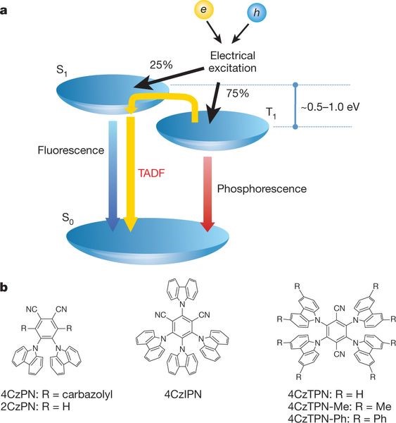
To ensure efficient RISC, TADF materials require a small singlet-triplet energy gap, corresponding to effective HOMO/LUMO separation. Hence, TADF materials typically adopt donor (D)-acceptor (A) or D-A-D structures to achieve HOMO/LUMO separation while maintaining transition oscillator strength.
Factors such as electronic properties of different donors/acceptors, triplet energy levels, structural rigidity, and distortion degree collectively influence ΔEST, oscillator strength, density of states, and exciton lifetime, ultimately determining the material’s photophysical properties and corresponding OLED device performance.
This topic uses the typical TADF molecule DPO-TXO2 as an example to demonstrate calculations for structural optimization, frequency analysis, single-point energy, excitation energy, spin-orbit coupling, etc. It also explains how to interpret data for result analysis, helping users gain deeper insights into BDF software usage.
Structural Optimization and Frequency Calculation
Generating Input Files for Structural Optimization and Frequency Analysis
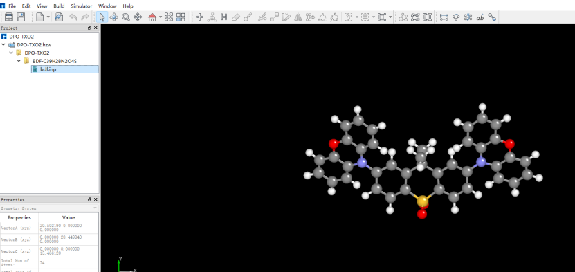
Import the prepared molecular structure DPO-TXO2.xyz into Device Studio to obtain the interface shown in Figure 1.1-1. Select Simulator → BDF → BDF, then configure parameters in the pop-up window.
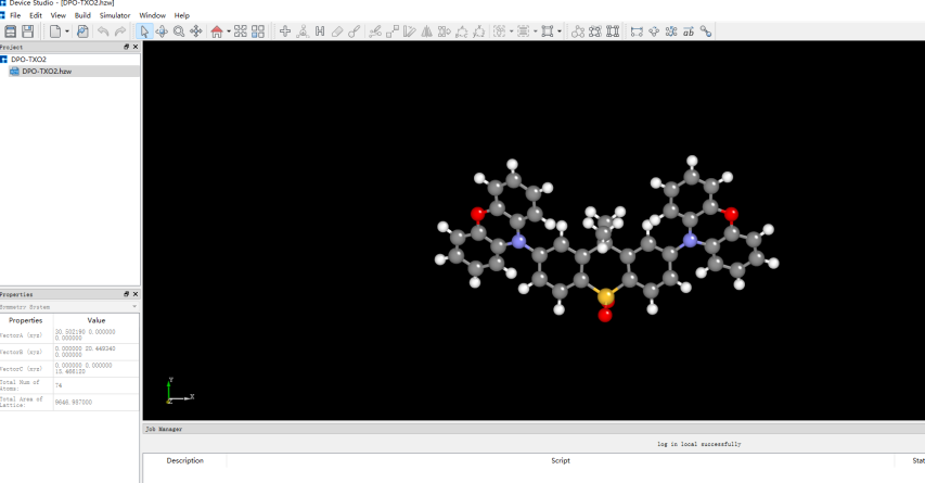
1.1-1
For structural optimization, select “Opt+Freq” as the calculation type. Users can set parameters such as method, functional, and basis set according to computational needs. For example, configure the Basic Settings panel as shown in Figure 1.1-2, deselect “Use MPEC+COSX” in the SCF panel (Figure 1.1-3), and retain default values for OPT and Freq panels. Click “Generate files” to create corresponding input files.
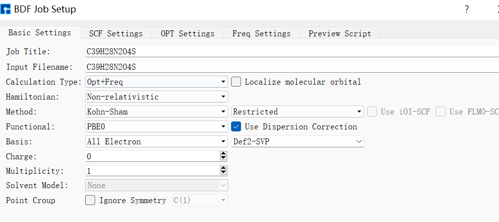
1.1-2
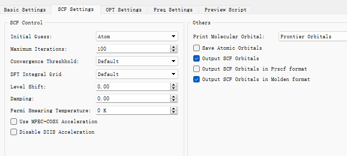
1.1-3
Key sections of the generated input file bdf.inp are shown below:
$compass
Title
  C39H28N2O4S
Geometry
C          3.86523        0.67704        0.08992
C          2.59676        1.19847       -0.21677
C          1.38236        0.46211       -0.14538
C          1.50274       -0.90633        0.05433
C          2.74673       -1.48909        0.32003
C          3.89360       -0.68925        0.41062
C          0.05129        1.23073       -0.21431
C         -1.26041        0.42556       -0.14322
C         -1.34326       -0.94957        0.03351
S          0.09634       -1.96093       -0.00226
C         -2.49139        1.13510       -0.19404
C         -3.75015        0.57230        0.07933
C         -3.75167       -0.80689        0.33485
C         -2.57699       -1.57032        0.24960
N          5.05789        1.50514        0.05106
N         -4.95552        1.38707        0.07338
C          5.09111        2.89319        0.50297
C          6.28464        3.63010        0.39676
O          7.47953        3.08357        0.01235
C          7.47002        1.78524       -0.41733
C          6.30967        0.99832       -0.48773
C          8.72243        1.30821       -0.82591
C          8.84826        0.02519       -1.33737
C          7.70856       -0.74821       -1.50329
C          6.45512       -0.24869       -1.12362
C          4.01062        3.58921        1.07620
C          4.07062        4.96296        1.37442
C          5.24860        5.67030        1.18784
C          6.36600        4.99303        0.72541
C         -6.19457        0.91553       -0.52385
C         -7.33964        1.73082       -0.48834
O         -7.34248        3.01488       -0.01720
C         -6.17443        3.51502        0.46887
C         -4.99409        2.75189        0.59422
C         -6.34490       -0.31630       -1.18638
C         -7.59189       -0.76699       -1.64640
C         -8.71481        0.03325       -1.52666
C         -8.57997        1.30489       -0.97531
C         -6.24475        4.86124        0.86098
C         -5.14195        5.49110        1.41274
C         -3.98465        4.75621        1.61916
C         -3.93157        3.39823        1.25512
O          0.11666       -2.61281       -1.29752
O          0.10373       -2.72112        1.23297
C          0.03300        2.06197       -1.51772
C          0.04308        2.16169        1.03932
H          2.54886        2.24058       -0.51595
H          2.82840       -2.56453        0.47286
H          4.82173       -1.17141        0.70878
H         -2.46593        2.19212       -0.44272
H         -4.67197       -1.32502        0.59460
H         -2.63456       -2.65479        0.35810
H          9.59544        1.95023       -0.74373
H          9.82187       -0.35477       -1.63187
H          7.78471       -1.74349       -1.93391
H          5.60034       -0.87480       -1.35499
H          3.08415        3.09348        1.32929
H          3.19316        5.47421        1.76453
H          5.30763        6.72822        1.42899
H          7.31255        5.51704        0.61863
H         -5.50297       -0.96874       -1.38412
H         -7.67454       -1.75102       -2.10194
H         -9.68032       -0.30389       -1.89032
H         -9.43942        1.96697       -0.92291
H         -7.17589        5.40700        0.73318
H         -5.19606        6.53771        1.70383
H         -3.11983        5.23203        2.07660
H         -3.02635        2.86997        1.52459
H          0.02919        1.39736       -2.38952
H          0.89268        2.72961       -1.61468
H         -0.84000        2.71525       -1.59635
H          0.04113        1.57168        1.96645
H         -0.82598        2.82200        1.07532
H          0.91163        2.82447        1.08397
End Geometry
Basis
  Def2-SVP
Skeleton
Group
  C(1)
$end

$bdfopt
Solver
  1
MaxCycle
  444
IOpt
  3
Hess
  final
$end

$xuanyuan
Direct
$end

$scf
RKS
Charge
  0
SpinMulti
  1
DFT
  PBE0
Molden
$end

$resp
Geom
$end
The Device Studio interface now appears as shown in Figure 1.1-4.
1.1-4
Note
Selecting “Opt+Freq” ensures identical conditions for structural optimization and frequency calculations. Separate Opt or Freq calculations are also possible.
Performing BDF Calculations
Before running BDF calculations, connect to a server with BDF installed (configuration details refer to Hongzhiyun Operation Guide).
After connecting to the server, users may review the input file parameters. If adjustments are needed, edit the file directly or regenerate it before executing BDF calculations.
In the interface shown in Figure 1.1-4, right-click bdf.inp → Run. Import the appropriate script in the pop-up window and click “Run” to submit the job (Figure 1.1-5).
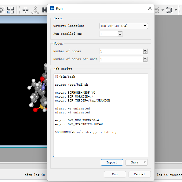
1.1-5
After calculation completes, click the download button to access results (Figure 1.1-6). Select the .out result file and click “Download”. (Job submission steps will not be reiterated in subsequent sections)
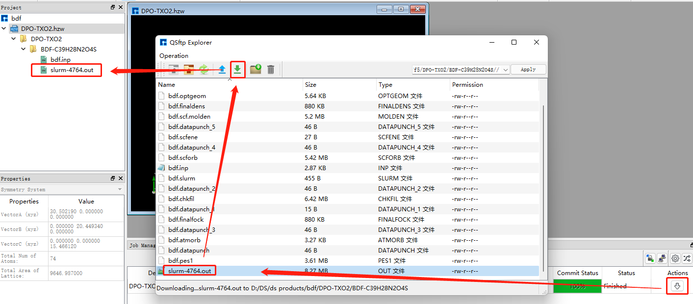
1.1-6
Analyzing Structural Optimization Results
Right-click the downloaded .out file and select “Open with/Open containing folder” to view results. Locate the convergence section:
               Force-RMS    Force-Max     Step-RMS     Step-Max
Conv. tolerance :  0.2000E-03   0.3000E-03   0.8000E-03   0.1200E-02
Current values  :  0.7369E-05   0.4013E-04   0.1843E-03   0.1041E-02
Geom. converge  :     Yes          Yes          Yes          Yes
When all four “Geom.converge” values are “Yes”, structural optimization has converged. Optimized Cartesian and internal coordinates appear above and below this section. The optimized coordinates can serve as initial structures for subsequent calculations.
Verify the absence of imaginary frequencies to confirm optimization reached a local minimum.
Single-Point Energy Calculation
Generating Single-Point Energy Input Files
Import optimized coordinates into Device Studio and rename to DPO-TXO2-sp.xyz (Figure 1.2-1).
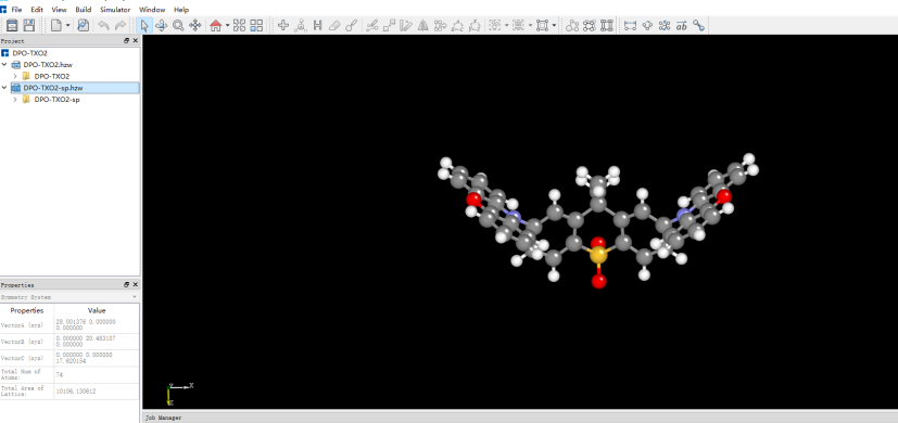
1.2-1
Select Simulator → BDF → BDF. In the pop-up window, choose “Single Point” (default) as calculation type. Configure parameters as needed (e.g., functional=PBE0, basis=Def2-TZVP). Retain other defaults and click “Generate files”. Key sections of bdf.inp:
$compass
Title
  C39H28N2O4S
Geometry
C       3.470732   -0.452949    0.333229
C       2.350276   -0.443126   -0.503378
C       1.255134   -1.275716   -0.258388
C       1.358849   -2.111496    0.851996
C       2.440432   -2.124490    1.711142
C       3.517727   -1.285828    1.451230
C      -0.000048   -1.278142   -1.147435
C      -1.255154   -1.275779   -0.258269
C      -1.358725   -2.111574    0.852120
S       0.000118   -3.243604    1.269861
C      -2.350358   -0.443230   -0.503130
C      -3.470738   -0.453151    0.333573
C      -3.517603   -1.286054    1.451551
C      -2.440223   -2.124643    1.711370
N       4.564102    0.414026    0.042506
N      -4.564206    0.413761    0.042962
C       4.451652    1.797113    0.288414
C       5.529066    2.638200   -0.032130
O       6.712474    2.137493   -0.580518
C       6.813862    0.759847   -0.795860
C       5.755871   -0.112762   -0.496962
C       7.999623    0.286590   -1.327509
C       8.161221   -1.076261   -1.582122
C       7.118160   -1.950624   -1.301513
C       5.922124   -1.471078   -0.764717
C       3.313452    2.367422    0.857787
C       3.242304    3.742953    1.084847
C       4.311909    4.564914    0.751035
C       5.460487    4.001069    0.193102
C      -5.755562   -0.112971   -0.497448
C      -6.813628    0.759568   -0.796285
O      -6.712738    2.137080   -0.579852
C      -5.529582    2.637766   -0.030885
C      -4.452105    1.796731    0.289592
C      -5.921333   -1.471159   -0.766141
C      -7.116971   -1.950658   -1.303865
C      -8.160095   -1.076369   -1.584473
C      -7.998981    0.286358   -1.328883
C      -5.461319    4.000541    0.194998
C      -4.313011    4.564332    0.753554
C      -3.243348    3.742416    1.087286
C      -3.314166    2.366978    0.859540
O       0.000119   -4.563841    0.371547
O       0.000187   -3.483649    2.840945
C      -0.000061   -2.561317   -2.024419
C      -0.000112   -0.071391   -2.097897
H       2.353966    0.240214   -1.341805
H       2.400109   -2.768057    2.584222
H       4.382110   -1.260026    2.103052
H      -2.354159    0.240153   -1.341521
H      -4.381950   -1.260326    2.103422
H      -2.399783   -2.768226    2.584432
H       8.781734    1.005474   -1.536628
H       9.092578   -1.440924   -1.998141
H       7.222431   -3.011204   -1.498846
H       5.108894   -2.153421   -0.550989
H       2.483350    1.726165    1.126879
H       2.346598    4.161499    1.529031
H       4.264620    5.633193    0.924336
H       6.321189    4.600814   -0.074686
H      -5.108047   -2.153429   -0.552391
H      -7.220889   -3.011140   -1.501914
H      -9.091141   -1.440996   -2.001221
H      -8.781175    1.005175   -1.537926
H      -6.322045    4.600258   -0.072770
H      -4.265977    5.632537    0.927382
H      -2.347852    4.160920    1.531932
H      -2.484014    1.725744    1.128541
H      -0.000061   -3.470168   -1.414898
H       0.891657   -2.554225   -2.661972
H      -0.891789   -2.554218   -2.661957
H      -0.000071    0.880895   -1.555239
H      -0.877870   -0.116199   -2.750591
H       0.877553   -0.116195   -2.750715
End Geometry
Basis
  Def2-TZVP
Skeleton
Group
  C(1)
$end

$xuanyuan
Direct
RS
  0.33
$end

$scf
RKS
Charge
  0
SpinMulti
  1
DFT
  CAM-B3LYP
MPEC+COSX
Molden
$end
Performing BDF Calculation
Following the same procedure as structural optimization: Right-click bdf.inp → Run → Verify script → Click “Run”. After completion, download the .out result file.
Analyzing Single-Point Energy Results
Open the downloaded .out file to locate key energy terms. E_tot represents total system energy (E_tot = E_ele + E_nn). In this example, E_tot = -2310.04883102 Hartree. Other terms: E_ele=electronic energy, E_nn=nuclear repulsion, E_1e=one-electron energy, E_ne=nuclear-electron attraction, E_kin=electron kinetic energy, E_ee=two-electron energy, E_xc=exchange-correlation energy.
Final scf result
E_tot =             -2311.25269871
E_ele =             -7827.28555013
E_nn  =              5516.03285142
E_1e  =            -14125.30142654
E_ne  =            -16425.97927385
E_kin =              2300.67784730
E_ee  =              6514.27065120
E_xc  =              -216.25477479
Virial Theorem      2.004596
Orbital occupation information follows, including energies and HOMO-LUMO gap. HOMO = -5.358 eV, LUMO = -1.962 eV, HOMO-LUMO gap = 3.396 eV. “Irrep” denotes irreducible representation (molecular orbital symmetry), both A for HOMO/LUMO in this case.
 [Final occupation pattern: ]

 Irreps:        A
 detailed occupation for iden/irep:      1   1
1.00 1.00 1.00 1.00 1.00 1.00 1.00 1.00 1.00 1.00
1.00 1.00 1.00 1.00 1.00 1.00 1.00 1.00 1.00 1.00
1.00 1.00 1.00 1.00 1.00 1.00 1.00 1.00 1.00 1.00
1.00 1.00 1.00 1.00 1.00 1.00 1.00 1.00 1.00 1.00
...
 Alpha   HOMO energy:      -0.24254414 au      -6.59996455 eV  Irrep: A
 Alpha   LUMO energy:      -0.04116321 au      -1.12010831 eV  Irrep: A
 HOMO-LUMO gap:       0.20138093 au       5.47985625 eV
The bottom sections show Mulliken/Lowdin population analyses and dipole moment:
   [Mulliken Population Analysis]
Atomic charges:
   1C      -0.0009
   2C      -0.3029
   3C       0.2227
   4C      -0.0143
   5C      -0.1228
   6C      -0.1890
   7C       0.0046
   8C       0.2227
   9C      -0.0150
  10S       0.7787
  11C      -0.3023
  12C      -0.0022
  13C      -0.1888
  14C      -0.1223
  15N      -0.0121
  16N      -0.0121
  17C       0.0563
  ...
   [Lowdin Population Analysis]
Atomic charges:
   1C      -0.1574
   2C      -0.0592
   3C      -0.0682
   4C      -0.2154
   5C      -0.1050
   6C      -0.0869
   7C      -0.2270
   8C      -0.0682
   9C      -0.2154
  10S       1.0012
  11C      -0.0591
  12C      -0.1574
  13C      -0.0869
  14C      -0.1050
  ...
  [Dipole moment: Debye]
           X          Y          Z         |u|
Elec:-.3535E+01 0.8441E-03 -.1954E+01
Nucl:-.1254E-12 -.4210E-12 -.2935E-13
Totl:   -3.5348     0.0008    -1.9541     4.0389
Viewing HOMO Orbital Diagrams
To better understand the electronic structure, frontier molecular orbital analysis is often required. The current BDF2022A release does not yet support post-processing data visualization. HOMO and LUMO orbital diagrams can be rendered using third-party software Multiwfn+VMD, requiring the scf.molden file. Usage methods are covered in dedicated posts on quantum chemistry forums and will not be addressed here.
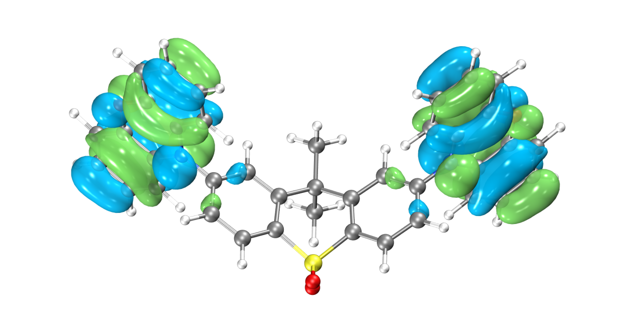
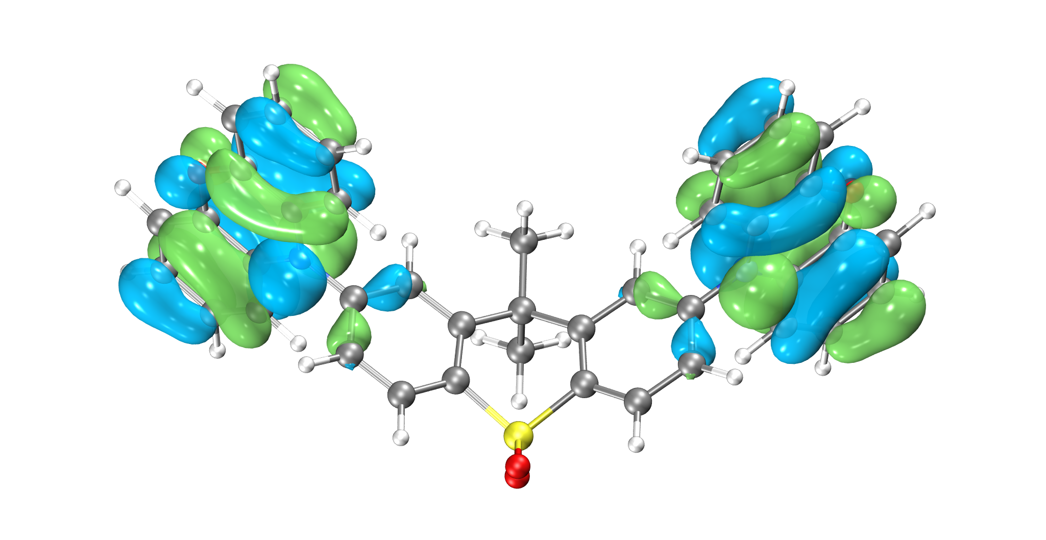
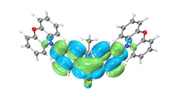
HOMO Orbital Distribution
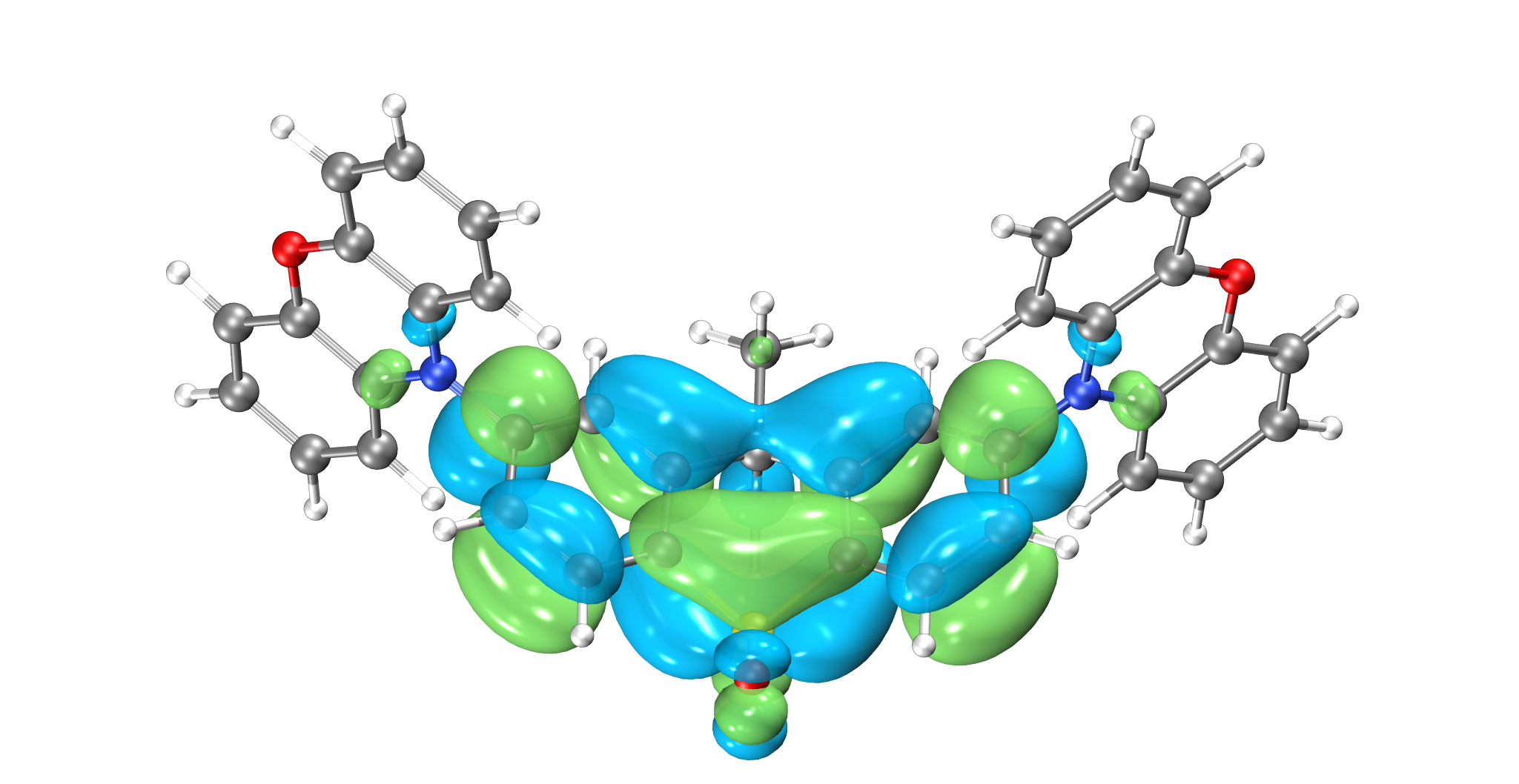
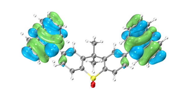
LUMO Orbital Distribution
The Highest Occupied Molecular Orbital (HOMO) and Lowest Unoccupied Molecular Orbital (LUMO) are shown above. The symmetrically distributed phenoxazine heterocycles on both sides are typical electron-donating structures, while the central sulfonated tetrahydronaphthalene is a typical electron-accepting structure. Thus, the entire molecule exhibits a classic D-A-D configuration. The HOMO orbital is primarily distributed on the wings, and the LUMO orbital is concentrated in the center, with minimal overlap between HOMO and LUMO orbitals—consistent with the electronic structural characteristics of TADF molecules. However, not all molecules with separated HOMO/LUMO orbitals exhibit TADF photoelectric properties; they must also satisfy the condition that both S1 and T1 excitations correspond to HOMO→LUMO orbital transitions. Therefore, we can further calculate the excited-state electronic structure of this molecule using BDF software.
Excited State Calculation
Generating Excited State Calculation Input Files
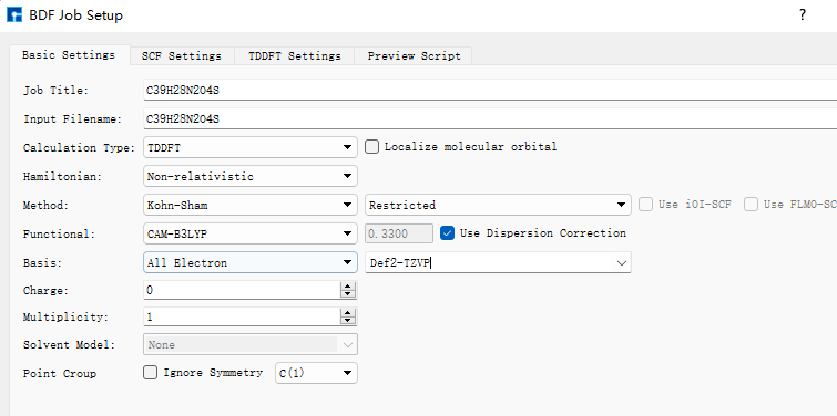
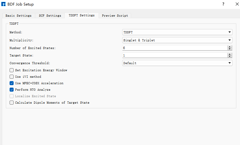
Using the optimized structure for TDDFT calculation: Right-click to copy the imported optimized structure and name it DPO-TXO2-td. Select TDDFT as the calculation type. Configure method, functional, basis set, etc., as needed. The previous single-point calculation showed clear HOMO-LUMO separation. For such distinctly D-A structured molecules, excited states often exhibit charge transfer characteristics. Thus, we select range-separated functionals most suitable for such systems, e.g., cam-B3LYP or ω-B97xd. Configure the Basic Settings panel as shown in Figure 1.3-1 and the TDDFT panel as in Figure 1.3-2. Click “Generate files” to create the input file.
1.3-1
1.3-2
Key sections of the generated bdf.inp file:
$compass
Title
  C39H28N2O4S
Geometry
C 3.56215000 -0.34631300 0.45361300
C 2.39970800 -0.43121500 -0.31807500
C 1.26327600 -1.11500900 0.12738900
C 1.35885600 -1.69579600 1.40258100
C 2.49771000 -1.60285400 2.19867100
C 3.61595700 -0.93278100 1.71813300
C 0.00021500 -1.24592200 -0.73874600
C -1.26297700 -1.11486500 0.12717900
C -1.35882900 -1.69562600 1.40235700
S -0.00010100 -2.61984500 2.07323100
C -2.39926700 -0.43096700 -0.31848800
C -3.56181100 -0.34590900 0.45301500
C -3.61589000 -0.93235000 1.71754500
C -2.49780200 -1.60255300 2.19826800
N 4.68577300 0.35565000 -0.05695800
N -4.68524700 0.35616500 -0.05781800
C 4.85522500 1.71734000 0.22325100
C 5.96987000 2.38879800 -0.31382300
O 6.88491700 1.74830700 -1.09915200
C 6.71947900 0.41903200 -1.36430000
C 5.62682300 -0.30753500 -0.85481400
C 7.67346300 -0.19823700 -2.15908800
C 7.56580700 -1.55645700 -2.46709500
C 6.49405000 -2.28575300 -1.96795600
C 5.53176100 -1.66610500 -1.16680600
C 3.96124200 2.44515800 1.01262100
C 4.17031100 3.80330200 1.26473400
C 5.27551600 4.45343400 0.73047600
C 6.17535900 3.73680700 -0.06194800
C -5.62705300 -0.30735400 -0.85450500
C -6.71928700 0.41938500 -1.36464300
O -6.88329900 1.74927200 -1.10167600
C -5.96897100 2.38946600 -0.31526500
C -4.85474100 1.71783400 0.22245400
C -5.53310000 -1.66639800 -1.16475900
C -6.49610200 -2.28636200 -1.96480800
C -7.56751800 -1.55693200 -2.46448300
C -7.67406700 -0.19823400 -2.15820200
C -6.17456800 3.73743100 -0.06324300
C -5.27514800 4.45388200 0.72982000
C -4.17031500 3.80359400 1.26465900
C -3.96122400 2.44545700 1.01253300
O -0.00015400 -3.96830000 1.50483700
O -0.00019500 -2.47109100 3.52665800
C 0.00020300 -2.64509100 -1.40495400
C 0.00034300 -0.20466000 -1.86117000
H 2.41118900 0.06372500 -1.28828500
H 2.48620300 -2.04935500 3.19547800
H 4.52498100 -0.84886800 2.31658900
H -2.41056900 0.06394100 -1.28871700
H -4.52499700 -0.84831800 2.31586200
H -2.48649200 -2.04903700 3.19508500
H 8.50056300 0.41098100 -2.52869800
H 8.32203900 -2.03354800 -3.09349600
H 6.39429300 -3.34933700 -2.19485600
H 4.69465500 -2.24580100 -0.77484200
H 3.09145400 1.94045700 1.43579900
H 3.45545900 4.34652000 1.88647900
H 5.44614600 5.51436800 0.92329600
H 7.05577600 4.20903800 -0.50207500
H -4.69625700 -2.24619000 -0.77237400
H -6.39717200 -3.35029700 -2.19042200
H -8.32431800 -2.03427800 -3.09000200
H -8.50081300 0.41112900 -2.52836600
H -7.05465600 4.20980200 -0.50387800
H -5.44580600 5.51480700 0.92266800
H -3.45579100 4.34667900 1.88689800
H -3.09175200 1.94062000 1.43619700
H 0.00013000 -3.45332000 -0.66309300
H 0.89243900 -2.75169300 -2.04060300
H -0.89196300 -2.75164000 -2.04071100
H 0.00033500 0.82736500 -1.47979800
H -0.87501100 -0.33812800 -2.51032400
H 0.87579000 -0.33816300 -2.51019000
End Geometry
Basis
  Def2-TZVP
Skeleton
Group
  C(1)
$end

$xuanyuan
Direct
RS
  0.33
$end

$scf
RKS
Charge
  0
SpinMulti
  1
DFT
  CAM-B3LYP
D3
MPEC+COSX
Molden
$end

$tddft
Imethod
  1
Isf
  0
Idiag
  1
Iroot
  6
MPEC+COSX
Istore
  1
$end

$tddft
NtoAnalyze
  0
$end

$tddft
Imethod
  1
Isf
  1
Idiag
  1
Iroot
  6
MPEC+COSX
Istore
  2
$end

$tddft
NtoAnalyze
  0
$end
Note
Files with identical names in Device Studio will be overwritten. Input files default to bdf.inp. To avoid data loss, create a new project for each calculation.
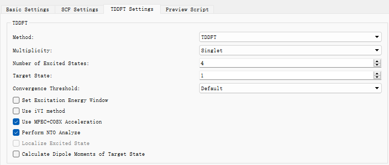
In the TDDFT panel, Method is generally recommended as TDDFT. Multiplicity can select singlet, triplet, or both. The default number of excited states calculated is 6. It is advisable to calculate 3 more states than needed (e.g., set to 13 for 10 desired states).
To perform NTO analysis, check “Perform NTO Analyze” in the TDDFT panel.
Performing BDF Calculation
After connecting to a server with BDF installed: Right-click bdf.inp → Run → Verify script → Click “Run”. After completion, download the .out result file.
Analyzing Excited State Results
Excitation Energy Analysis
Open the downloaded .out file to locate excitation energies, oscillator strengths, and transition dipole moments. isf=0 indicates singlet excited state information; isf=1 indicates triplet excited state information.
      No. Pair   ExSym   ExEnergies     Wavelengths      f     D<S^2>          Dominant Excitations             IPA   Ova     En-E1

    1   A    2   A    3.4840 eV        355.86 nm   0.0023   0.0000  69.9%  CV(0):   A( 162 )->   A( 163 )   5.584 0.164    0.0000
    2   A    3   A    3.4902 eV        355.24 nm   0.0005   0.0000  69.3%  CV(0):   A( 161 )->   A( 163 )   5.592 0.167    0.0061
    3   A    4   A    3.8143 eV        325.05 nm   0.0003   0.0000  31.6%  CV(0):   A( 162 )->   A( 164 )   6.182 0.482    0.3302
    4   A    5   A    3.8152 eV        324.97 nm   0.0040   0.0000  31.0%  CV(0):   A( 161 )->   A( 164 )   6.189 0.485    0.3312
    5   A    6   A    4.1185 eV        301.05 nm   0.0163   0.0000  30.7%  CV(0):   A( 161 )->   A( 168 )   6.944 0.583    0.6344
    6   A    7   A    4.1229 eV        300.72 nm   0.1369   0.0000  30.8%  CV(0):   A( 162 )->   A( 168 )   6.936 0.582    0.6388

 *** Ground to excited state Transition electric dipole moments (Au) ***
    State          X           Y           Z          Osc.
       1       0.0003      -0.1642       0.0004       0.0023
       2       0.0579      -0.0010       0.0549       0.0005
       3       0.0019       0.0580      -0.0012       0.0003
       4      -0.1789       0.0007       0.1034       0.0040
       5      -0.0070      -0.4020       0.0039       0.0163
       6       1.0339      -0.0028      -0.5353       0.1369

    ---------------------------------------------
    ---- End TD-DFT Calculations for isf = 0 ----
...
  No. Pair   ExSym   ExEnergies     Wavelengths      f     D<S^2>          Dominant Excitations             IPA   Ova     En-E1

    1   A    1   A    2.7522 eV        450.49 nm   0.0000   2.0000  25.3%  CV(1):   A( 162 )->   A( 167 )   6.920 0.659    0.0000
    2   A    2   A    2.7522 eV        450.49 nm   0.0000   2.0000  25.1%  CV(1):   A( 161 )->   A( 167 )   6.928 0.659    0.0000
    3   A    3   A    3.3404 eV        371.17 nm   0.0000   2.0000  33.1%  CV(1):   A( 154 )->   A( 163 )   8.200 0.672    0.5882
    4   A    4   A    3.3862 eV        366.15 nm   0.0000   2.0000  20.9%  CV(1):   A( 154 )->   A( 165 )   8.983 0.649    0.6340
    5   A    5   A    3.4620 eV        358.13 nm   0.0000   2.0000  50.3%  CV(1):   A( 162 )->   A( 163 )   5.584 0.322    0.7098
    6   A    6   A    3.4757 eV        356.72 nm   0.0000   2.0000  32.5%  CV(1):   A( 161 )->   A( 163 )   5.592 0.466    0.7235

 *** Transition dipole moments (Au) ***
    State          X           Y           Z          Osc.
       1-6: All 0.0000 (spin-forbidden transitions)

    ---------------------------------------------
    ---- End TD-DFT Calculations for isf = 1 ----
Results are summarized in the table below:
The table lists excited states in ascending energy order, including multiplicity, irreducible representation, dominant electron-hole pair excitations, excitation energy, oscillator strength, transition orbital contribution percentage, dipole moment, wavelength, and absolute overlap integral. It shows that the six calculated singlet excited states have energies between 2.7-4.0 eV, densely distributed. The first two singlet excited states have wavelengths around 355 nm, primarily involving HOMO→LUMO and HOMO-1→LUMO transitions, exhibiting charge transfer characteristics.
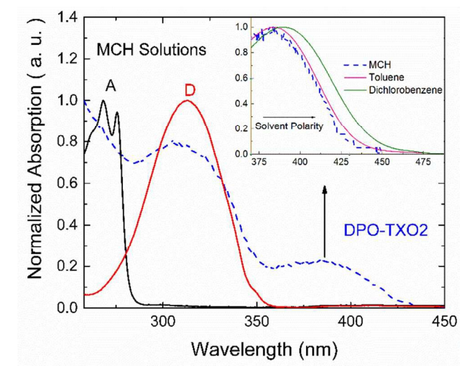
Literature reports indicate that DPO-TXO2’s lowest absorption peak in solvent environments is around 380 nm, red-shifting with increasing solvent polarity. This occurs because higher polarity solvents stabilize more polar excited states to a greater extent. n-orbitals have the highest polarity, followed by π*, while π-orbitals have the lowest polarity.
Calculations show DPO-TXO2’s ground state dipole moment is 2.842 D, while the S1 excited state dipole moment is 19.4 D. The significantly larger excited state dipole moment leads to greater stabilization through electrostatic interactions with the solvent environment compared to the ground state, resulting in a red shift of the absorption spectrum.
NTO Analysis
After excited state calculations, Natural Transition Orbital (NTO) analysis can provide clearer insights into transition characteristics. Readers interested in NTO principles may refer to relevant articles (http://sobereva.com/91).
To analyze the S1 state specifically: Configure the Basic Settings panel as in Figure 1.3-1 and check “Perform NTO Analyze” in the TDDFT panel (Figure 1.3-6).
1.3-6
Note
The second tddft module in the input file can also be manually modified as:
$tddft
NtoAnalyze
  1       # NTO analysis for one state
  1       # Specify the first excited state
$end
After calculation, an nto1_1.molden file is generated containing NTO orbital information instead of MO orbitals. Process this file using Multiwfn (main function 0 with adjusted orbital info) to obtain NTO eigenvalues and orbital diagrams. Usage details are covered in specialized forum posts and won’t be discussed here.
DPO-TXO2’s S1 excitation requires two sets of NTO orbitals for adequate description. Below are VMD-rendered hole-particle orbital pairs:
Hole1 → particle1 (73.26%)
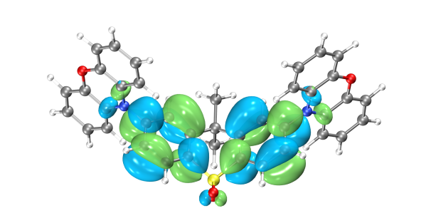
Hole2 → particle2 (26.59%)
NTO analysis reveals the dominant transition is Hole1→particle1 (73.26%), followed by Hole2→particle2 (26.59%). Electrons transition from phenoxazine donor groups on both sides to the central acceptor group in the S1 excited state.
Absorption Spectrum Analysis
To theoretically predict absorption spectra, excite states are broadened using Gaussian functions. After TDDFT calculation, execute the plotspec.py script from the BDF installation path via terminal. For Hongzhiyun Cloud users, terminal access methods are covered in the user guide (not discussed here).
Run $BDFHOME/sbin/plotspec.py bdf.out to generate bdf.stick.csv (stick spectrum data) and bdf.spec.csv (Gaussian-broadened spectrum, default FWHM=0.5 eV). Plot bdf.spec.csv using Origin:
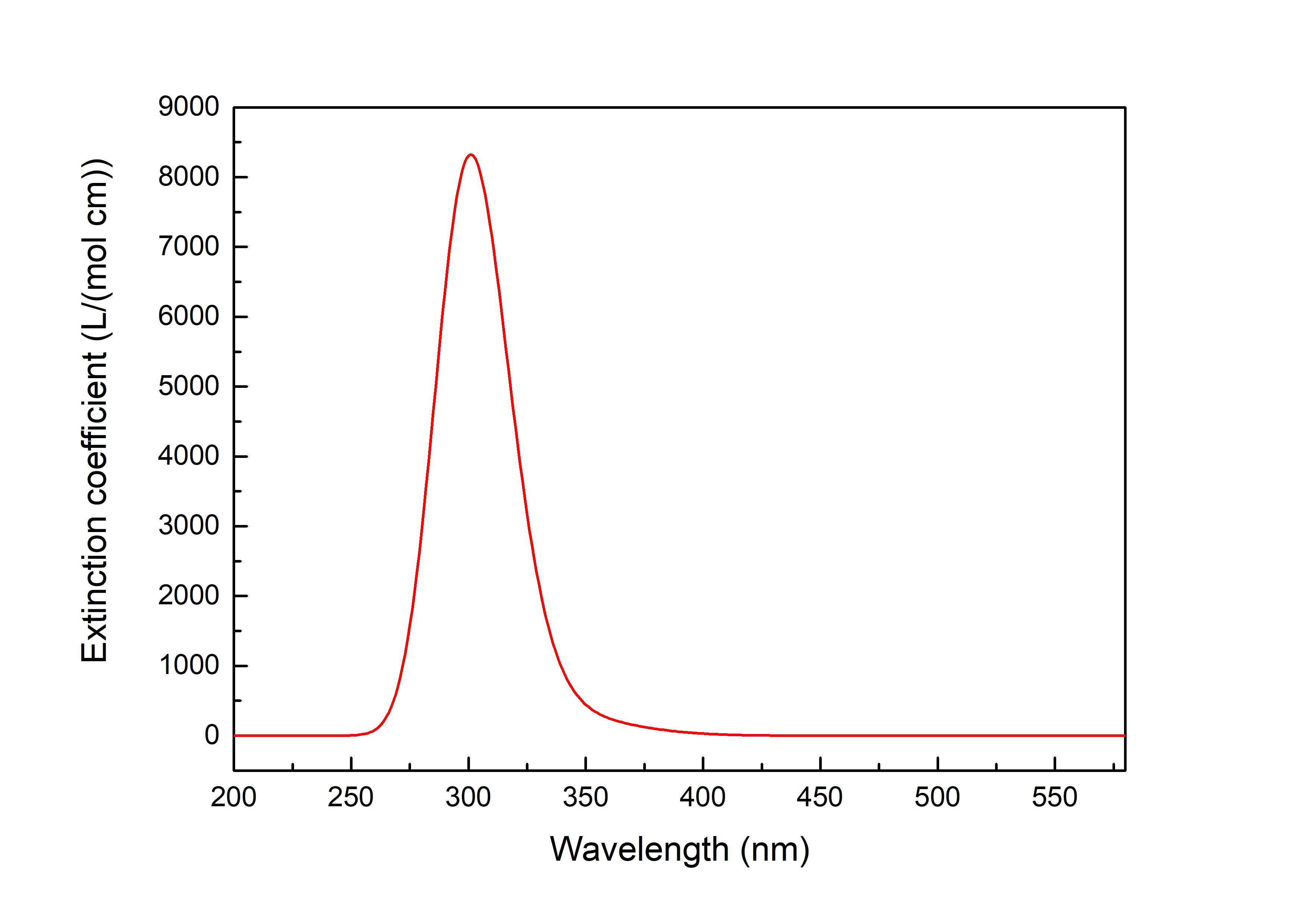
This indicates electrons in the ground state are most likely to absorb 300 nm light for transitions.
Excited State Optimization
Generating Excited State Optimization Input Files
Import the optimized ground state structure. Select TDDFT-OPT as calculation type with PBE0 functional and Def2-SVP basis set. Configure Basic Settings as in Figure 1.4-1 and disable “Use MPEC+COSX” in the SCF panel (Figure 1.1-3). For S1 optimization: Set multiplicity to Singlet and Target State to 1 in the TDDFT panel, checking “Calculate Dipole Moments of Target State” (Figure 1.4-2). Keep OPT panel defaults and click “Generate files”.
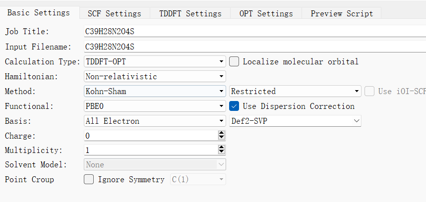
1.4-1
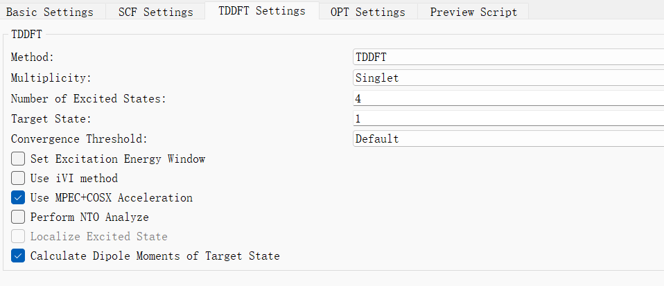
1.4-2
Generated bdf.inp parameters:
$compass
Title
  C39H28N2O4S
Geometry
C 3.56215000 -0.34631300 0.45361300
C 2.39970800 -0.43121500 -0.31807500
C 1.26327600 -1.11500900 0.12738900
C 1.35885600 -1.69579600 1.40258100
C 2.49771000 -1.60285400 2.19867100
C 3.61595700 -0.93278100 1.71813300
C 0.00021500 -1.24592200 -0.73874600
C -1.26297700 -1.11486500 0.12717900
C -1.35882900 -1.69562600 1.40235700
S -0.00010100 -2.61984500 2.07323100
C -2.39926700 -0.43096700 -0.31848800
C -3.56181100 -0.34590900 0.45301500
C -3.61589000 -0.93235000 1.71754500
C -2.49780200 -1.60255300 2.19826800
N 4.68577300 0.35565000 -0.05695800
N -4.68524700 0.35616500 -0.05781800
C 4.85522500 1.71734000 0.22325100
C 5.96987000 2.38879800 -0.31382300
O 6.88491700 1.74830700 -1.09915200
C 6.71947900 0.41903200 -1.36430000
C 5.62682300 -0.30753500 -0.85481400
C 7.67346300 -0.19823700 -2.15908800
C 7.56580700 -1.55645700 -2.46709500
C 6.49405000 -2.28575300 -1.96795600
C 5.53176100 -1.66610500 -1.16680600
C 3.96124200 2.44515800 1.01262100
C 4.17031100 3.80330200 1.26473400
C 5.27551600 4.45343400 0.73047600
C 6.17535900 3.73680700 -0.06194800
C -5.62705300 -0.30735400 -0.85450500
C -6.71928700 0.41938500 -1.36464300
O -6.88329900 1.74927200 -1.10167600
C -5.96897100 2.38946600 -0.31526500
C -4.85474100 1.71783400 0.22245400
C -5.53310000 -1.66639800 -1.16475900
C -6.49610200 -2.28636200 -1.96480800
C -7.56751800 -1.55693200 -2.46448300
C -7.67406700 -0.19823400 -2.15820200
C -6.17456800 3.73743100 -0.06324300
C -5.27514800 4.45388200 0.72982000
C -4.17031500 3.80359400 1.26465900
C -3.96122400 2.44545700 1.01253300
O -0.00015400 -3.96830000 1.50483700
O -0.00019500 -2.47109100 3.52665800
C 0.00020300 -2.64509100 -1.40495400
C 0.00034300 -0.20466000 -1.86117000
H 2.41118900 0.06372500 -1.28828500
H 2.48620300 -2.04935500 3.19547800
H 4.52498100 -0.84886800 2.31658900
H -2.41056900 0.06394100 -1.28871700
H -4.52499700 -0.84831800 2.31586200
H -2.48649200 -2.04903700 3.19508500
H 8.50056300 0.41098100 -2.52869800
H 8.32203900 -2.03354800 -3.09349600
H 6.39429300 -3.34933700 -2.19485600
H 4.69465500 -2.24580100 -0.77484200
H 3.09145400 1.94045700 1.43579900
H 3.45545900 4.34652000 1.88647900
H 5.44614600 5.51436800 0.92329600
H 7.05577600 4.20903800 -0.50207500
H -4.69625700 -2.24619000 -0.77237400
H -6.39717200 -3.35029700 -2.19042200
H -8.32431800 -2.03427800 -3.09000200
H -8.50081300 0.41112900 -2.52836600
H -7.05465600 4.20980200 -0.50387800
H -5.44580600 5.51480700 0.92266800
H -3.45579100 4.34667900 1.88689800
H -3.09175200 1.94062000 1.43619700
H 0.00013000 -3.45332000 -0.66309300
H 0.89243900 -2.75169300 -2.04060300
H -0.89196300 -2.75164000 -2.04071100
H 0.00033500 0.82736500 -1.47979800
H -0.87501100 -0.33812800 -2.51032400
H 0.87579000 -0.33816300 -2.51019000
End Geometry
Basis
  Def2-TZVP
Skeleton
Group
  C(1)
$end

$bdfopt
Solver
  1
MaxCycle
  444
IOpt
  3
$end

$xuanyuan
Direct
$end

$scf
RKS
Charge
  0
SpinMulti
  1
DFT
  PBE0
D3
Molden
$end

$tddft
Imethod
  1
Isf
  0
Ialda
  4
Idiag
  1
Iroot
  4
MPEC+COSX
Istore
  1
$end

$resp
Geom
Method
  2
Nfiles
  1
Iroot
  1
$end
Note
For T1 optimization: Change multiplicity to Triplet in the TDDFT panel while keeping other parameters identical to S1 optimization.
Performing BDF Calculation
After connecting to a BDF server: Right-click bdf.inp → Run → Verify script → Click “Run”. Download the .out result file after completion.
Analyzing Excited State Optimization Results Open the .out file. Convergence is confirmed when all four Geom.converge values are “YES” (similar to ground state optimization). The energy difference between optimized T1 and S1 gives ΔEST ≈ 2.425 eV.
Spin-Orbit Coupling Calculation
Generating Spin-Orbit Coupling Input Files
Perform SOC calculation on optimized structures. Select TDDFT-SOC as calculation type with sf-x2c Hamiltonian. Choose relativistic basis sets (e.g., cc-pVDZ-DK). Configure Basic Settings as in Figure 1.5-1, keeping SCF/TDDFT panels at defaults. Click “Generate files”.
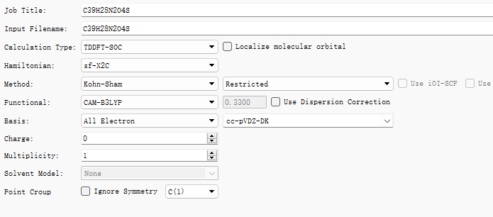
1.5-1
Generated bdf.inp parameters:
$compass
Title
  C39H28N2O4S
Geometry
C 3.56214999 -0.34631300 0.45361300
C 2.39970799 -0.43121500 -0.31807500
C 1.26327600 -1.11500899 0.12738900
C 1.35885600 -1.69579600 1.40258100
C 2.49771000 -1.60285400 2.19867100
C 3.61595699 -0.93278100 1.71813299
C 0.00021500 -1.24592199 -0.73874600
C -1.26297700 -1.11486500 0.12717899
C -1.35882900 -1.69562600 1.40235700
S -0.00010100 -2.61984500 2.07323099
C -2.39926700 -0.43096700 -0.31848800
C -3.56181100 -0.34590900 0.45301500
C -3.61588999 -0.93235000 1.71754500
C -2.49780200 -1.60255299 2.19826800
N 4.68577300 0.35565000 -0.05695800
N -4.68524700 0.35616500 -0.05781800
C 4.85522499 1.71734000 0.22325100
C 5.96987000 2.38879800 -0.31382300
O 6.88491699 1.74830700 -1.09915199
C 6.71947899 0.41903200 -1.36430000
C 5.62682299 -0.30753500 -0.85481400
C 7.67346299 -0.19823700 -2.15908800
C 7.56580700 -1.55645700 -2.46709500
C 6.49404999 -2.28575300 -1.96795600
C 5.53176100 -1.66610499 -1.16680600
C 3.96124200 2.44515800 1.01262099
C 4.17031099 3.80330200 1.26473400
C 5.27551599 4.45343399 0.73047600
C 6.17535900 3.73680700 -0.06194800
C -5.62705300 -0.30735400 -0.85450500
C -6.71928699 0.41938500 -1.36464300
O -6.88329900 1.74927200 -1.10167600
C -5.96897099 2.38946600 -0.31526500
C -4.85474099 1.71783400 0.22245400
C -5.53310000 -1.66639800 -1.16475900
C -6.49610199 -2.28636200 -1.96480800
C -7.56751799 -1.55693200 -2.46448300
C -7.67406700 -0.19823400 -2.15820200
C -6.17456799 3.73743100 -0.06324299
C -5.27514799 4.45388200 0.72982000
C -4.17031500 3.80359399 1.26465899
C -3.96122400 2.44545700 1.01253299
O -0.00015400 -3.96830000 1.50483700
O -0.00019500 -2.47109099 3.52665799
C 0.00020300 -2.64509099 -1.40495400
C 0.00034300 -0.20466000 -1.86117000
H 2.41118899 0.06372500 -1.28828499
H 2.48620300 -2.04935499 3.19547800
H 4.52498100 -0.84886800 2.31658900
H -2.41056900 0.06394100 -1.28871699
H -4.52499699 -0.84831800 2.31586200
H -2.48649200 -2.04903700 3.19508500
H 8.50056299 0.41098100 -2.52869799
H 8.32203900 -2.03354800 -3.09349600
H 6.39429300 -3.34933699 -2.19485600
H 4.69465500 -2.24580100 -0.77484200
H 3.09145400 1.94045700 1.43579900
H 3.45545899 4.34651999 1.88647900
H 5.44614599 5.51436800 0.92329600
H 7.05577599 4.20903799 -0.50207500
H -4.69625700 -2.24618999 -0.77237400
H -6.39717200 -3.35029699 -2.19042199
H -8.32431799 -2.03427800 -3.09000200
H -8.50081300 0.41112900 -2.52836600
H -7.05465599 4.20980199 -0.50387800
H -5.44580600 5.51480700 0.92266800
H -3.45579100 4.34667899 1.88689800
H -3.09175200 1.94062000 1.43619699
H 0.00012999 -3.45332000 -0.66309300
H 0.89243900 -2.75169300 -2.04060299
H -0.89196300 -2.75164000 -2.04071099
H 0.00033500 0.82736500 -1.47979799
H -0.87501100 -0.33812800 -2.51032400
H 0.87579000 -0.33816300 -2.51019000
End Geometry
Basis
  cc-pVDZ-DK
Skeleton
Group
  C(1)
$end

$xuanyuan
Heff
  21
Hsoc
  2
Direct
RS
  0.33
$end

$scf
RKS
Charge
  0
SpinMulti
  1
DFT
  CAM-B3LYP
D3
MPEC+COSX
Molden
$end

$tddft
Imethod
  1
Isf
  0
Idiag
  1
Iroot
  6
MPEC+COSX
Istore
  1
$end

$tddft
Imethod
  1
Isf
  1
Idiag
  1
Iroot
  6
MPEC+COSX
Istore
  2
$end

$tddft
Isoc
  2
Nfiles
  2
Imatsoc
  -1
Imatrsf
  -1
Imatrso
  -1
$end
Performing BDF Calculation
After connecting to a BDF server: Right-click bdf.inp → Run → Verify script → Click “Run”. Download the .out result file after completion.
Spin-Orbit Coupling Matrix Element Analysis
Open the .out file. SOC matrix elements are printed under “Print selected matrix elements of [Hsoc]”:
 SocPairNo. =    8   SOCmat = <  0  0  0 |Hso|  2  1  1 >     Dim =    1    3
   mi/mj          ReHso(au)       cm^-1               ImHso(au)       cm^-1
  0.0 -1.0     -0.0000018883     -0.4144393040     -0.0000012470     -0.2736747987
  0.0  0.0      0.0000000000      0.0000000000     -0.0000076582     -1.6807798007
  0.0  1.0     -0.0000018883     -0.4144393040      0.0000012470      0.2736747987

 SocPairNo. =    9   SOCmat = <  0  0  0 |Hso|  2  1  2 >     Dim =    1    3
   mi/mj          ReHso(au)       cm^-1               ImHso(au)       cm^-1
  0.0 -1.0      0.0000038630      0.8478326909     -0.0000006073     -0.1332932016
  0.0  0.0      0.0000000000      0.0000000000     -0.0000037537     -0.8238381363
  0.0  1.0      0.0000038630      0.8478326909      0.0000006073      0.1332932016
...
Tabulated results:
|SOC| (cm⁻¹) |
T1 |
T2 |
|---|---|---|
S0 |
1.822 |
1.467 |
S1 |
0.522 |
0.842 |
The calculated SOC between S0 and T1 is 1.822 cm⁻¹. If the energy gap is sufficiently small, this facilitates intersystem crossing.
BDF-QM/MM Case Tutorial I
This topic introduces a quantum chemistry and molecular mechanics combined method (QM/MM method), which incorporates the accuracy of quantum chemistry and the efficiency of molecular mechanics. The core idea is to treat the region of interest with quantum mechanics while handling the remaining parts with classical molecular mechanics.
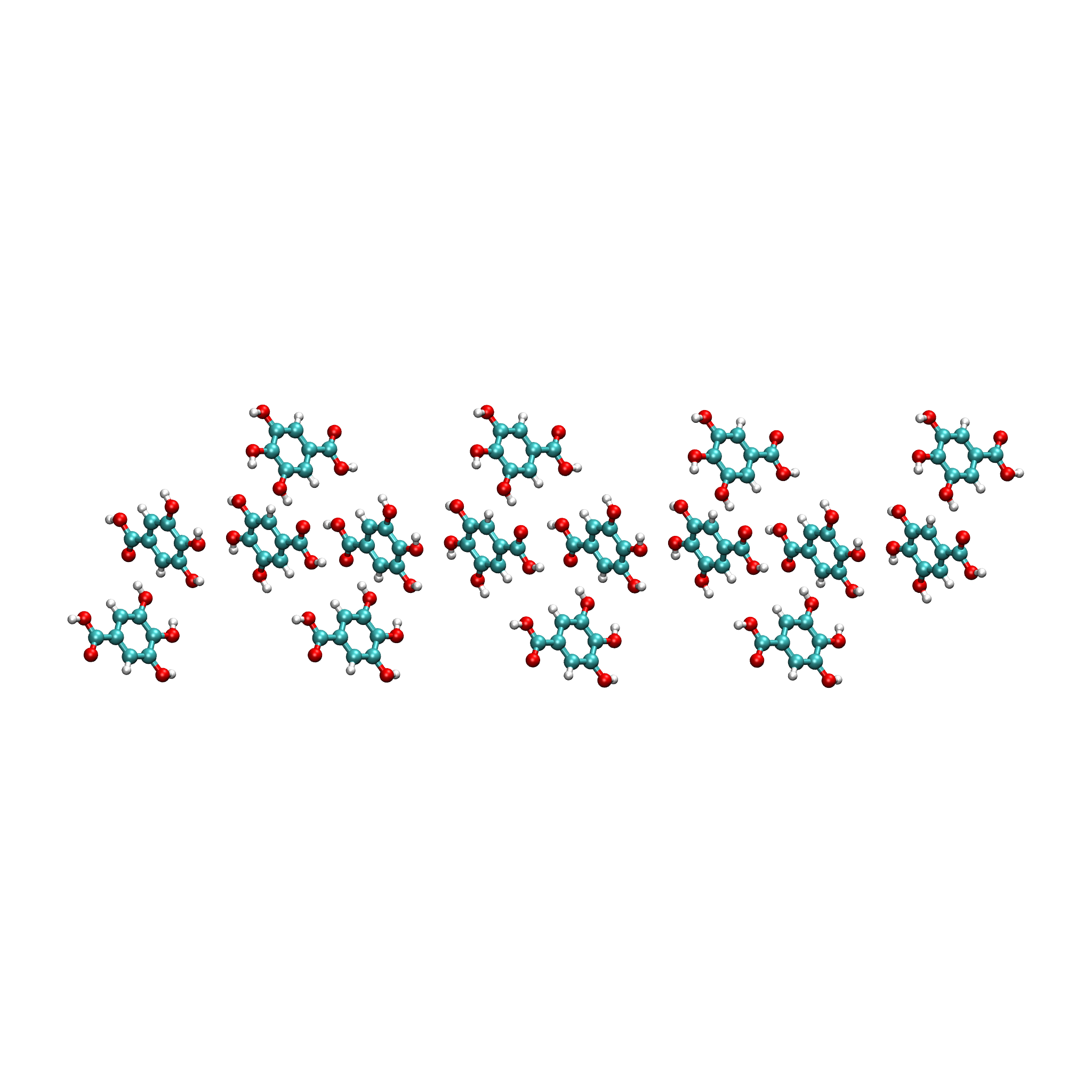
This chapter uses a typical gallic acid molecule (Gallic Acid, GA) as an example to cover input file preparation, QM/MM single-point calculations, QM/MM structural optimization, and QM/MM excited-state calculations. The BDF program primarily handles the quantum chemistry calculations, while the modified pDynamo2.0 package developed by the BDF team manages the remaining tasks. The tutorial also explains how to read data for result analysis, helping users gain a deeper understanding of BDF software usage.
Input File Preparation
Generally, molecular dynamics simulations are required before QM/MM calculations to obtain suitable initial conformations. When using PDB, MOL2, or xyz files as input, the pDynamo2.0 package only supports the OPLS force field. For small molecules and non-standard amino acids, force field parameters may be incomplete, so this approach is not recommended. Amber is preferred, using topology files to input force field parameters. Using Amber as an example, extract structures of interest from the dynamics simulation trajectory and store them in a .crd file. This file, along with the corresponding parameter/topology file .prmtop, serves as the starting point for QM/MM calculations. The Python script is as follows:
from pBabel import AmberCrdFile_ToCoordinates3, AmberTopologyFile_ToSystem
# Read input information
molecule  = AmberTopologyFile_ToSystem (Topfile)
molecule.coordinates3 = AmberCrdFile_ToCoordinates3(CRDfile)
Prerequisites: Install AmberTools and Python 2.0, and correctly set the AMBERHOME and PDYNAMO environment variables. To generate the coordinate file GallicAcid.crd and parameter/topology file GallicAcid.prmop from the initial structure file GallicAcid.pdb (Figure 1, unit cell 2 * 1 * 1), follow these steps:
Run the antechamber program to convert the Pdb file to a mol2 file:
antechamber -i GallicAcid.pdb -fi pdb -o GallicAcid.mol2 -fo mol2 -j 5 -at amber -dr no - -i specifies the input file - -fi specifies the input file type - -o specifies the output file - -fo specifies the output file type - -j matches atom and bond types - -at defines atom types
Run the parmchk2 program to generate the force field parameter file for the system:
parmchk2 -i GallicAcid.mol2 -f mol2 -o GallicAcid.frcmod
Run the tleap program to build the system topology and define force field parameters:
Start the tleap program using the tleap command:
-I: Adding /es01/jinan/hzw001/home/hzw1011/anaconda3/envs/AmberTools21/dat/leap/prep to search path.
-I: Adding /es01/jinan/hzw001/home/hzw1011/anaconda3/envs/AmberTools21/dat/leap/lib to search path.
-I: Adding /es01/jinan/hzw001/home/hzw1011/anaconda3/envs/AmberTools21/dat/leap/parm to search path.
-I: Adding /es01/jinan/hzw001/home/hzw1011/anaconda3/envs/AmberTools21/dat/leap/cmd to search path.

Welcome to LEaP!
(no leaprc in search path)
>
Identify and load the system force field: source leaprc.gaff (this is the GAFF force field):
> source leaprc.gaff
----- Source: /es01/jinan/hzw001/home/hzw1011/anaconda3/envs/AmberTools21/dat/leap/cmd/leaprc.gaff
----- Source of /es01/jinan/hzw001/home/hzw1011/anaconda3/envs/AmberTools21/dat/leap/cmd/leaprc.gaff done
Log file: ./leap.log
Loading parameters: /es01/jinan/hzw001/home/hzw1011/anaconda3/envs/AmberTools21/dat/leap/parm/gaff.dat
Reading title:
AMBER General Force Field for organic molecules (Version 1.81, May 2017)
>
Load the ligand mol2 file: GA = loadmol2 GallicAcid.mol2:
> GA = loadmol2 GallicAcid.mol2
Loading Mol2 file: ./GallicAcid.mol2
Reading MOLECULE named WAT
>
Check if the imported structure is accurate or missing parameters: check GA
Load the system molecule template and complete missing parameters: loadamberparams GallicAcid.frcmod
Prepare the generated Sustiva library file: saveoff GA GallicAcid.lib
Modify the generated Sustiva library file and load it: loadoff GallicAcid.lib
> loadoff GallicAcid.lib
Loading library: ./GallicAcid.lib
Save the .crd and .prmop files: saveamberparm GA GallicAcid.prmtop GallicAcid.crd
> saveamberparm GA GallicAcid.prmtop GallicAcid.crd
Checking Unit.
Building topology.
Building atom parameters.
Building bond parameters.
Building angle parameters.
Building proper torsion parameters.
Building improper torsion parameters.
 total 112 improper torsions applied
Building H-Bond parameters.
Incorporating Non-Bonded adjustments.
Not Marking per-residue atom chain types.
Marking per-residue atom chain types.
  (Residues lacking connect0/connect1 -
   these don't have chain types marked:

        res     total affected

        WAT     1
  )
 (no restraints)
>
Exit the tleap program: quit
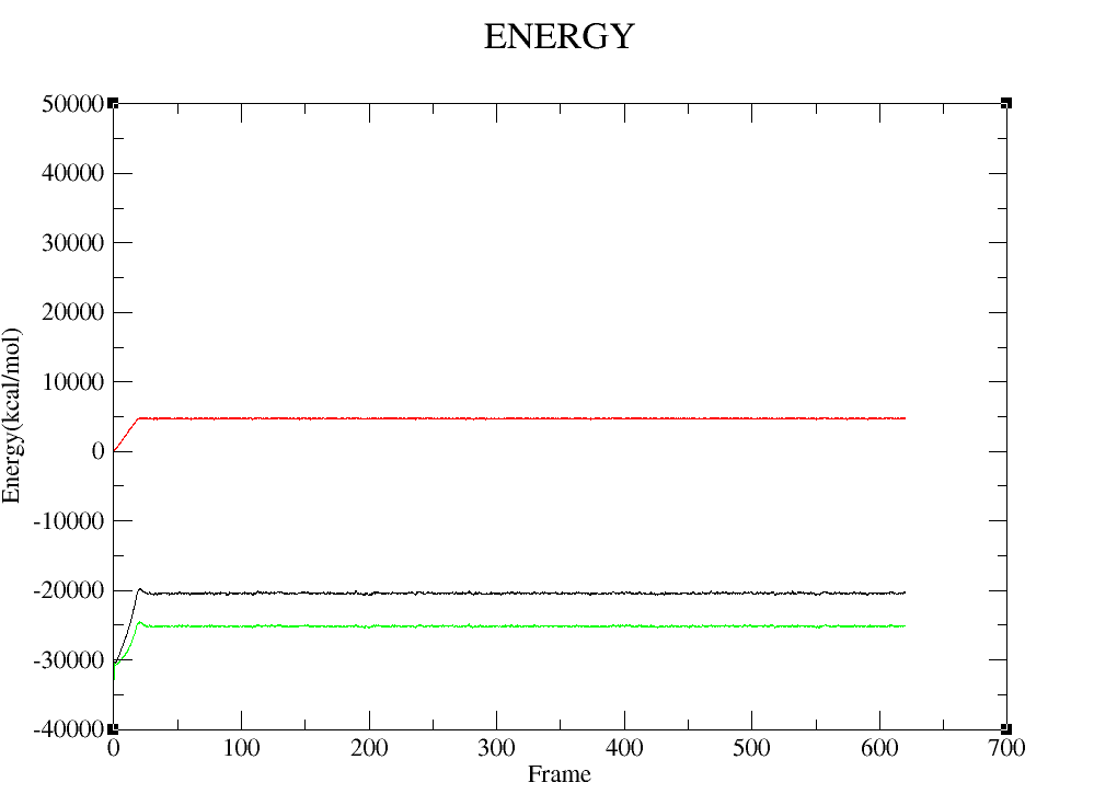
Molecular Dynamics Simulation
Use Amber software for molecular dynamics simulation. First, perform energy minimization on the system. The input file min.in is as follows:
   Initial minimisation of GallicAcid complex
    &cntrl
     imin=1, maxcyc=200, ncyc=50,
     cut=16, ntb=0, igb=1,
   &end
- imin=1: Run energy minimization
- maxcyc=200: Maximum number of minimization cycles
- ncyc=50: Use steepest descent algorithm for cycles 0 to ncyc, then switch to conjugate gradient for cycles ncyc to maxcyc
- cut=16: Non-bonded cutoff distance in Å
- ntb=0: Turn off periodic boundary conditions
- igb=1: Born model
Run energy minimization with the following command:
sander -O -i min.in -o GallicAcid_min.out -p GallicAcid.prmtop -c GallicAcid.crd -r GallicAcid_min.rst &
Where GallicAcid_min.rst is the output restart file containing coordinates and velocities.
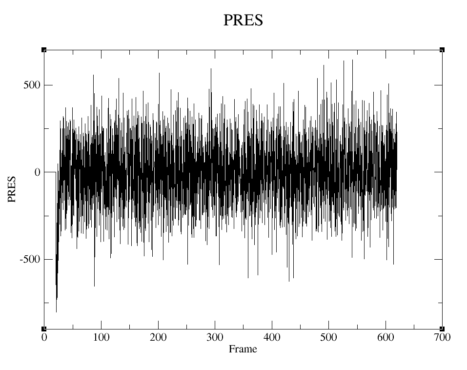
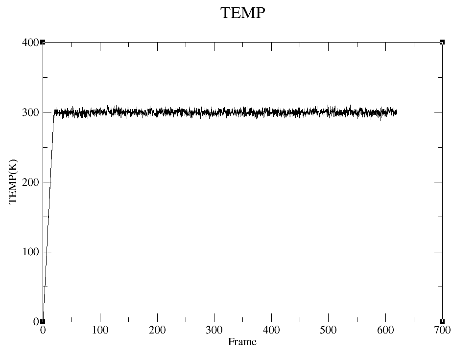
Use the restart file from minimization to heat the system and complete molecular dynamics simulation. The input file md.in is as follows:
Initial MD equilibration
 &cntrl
  imin=0, irest=0,
  nstlim=1000,dt=0.001, ntc=1,
  ntpr=20, ntwx=20,
  cut=16, ntb=0, igb=1,
  ntt=3, gamma_ln=1.0,
  tempi=0.0, temp0=300.0,
&end
imin=0: Perform molecular dynamics (MD)
irest=0: Read coordinates and velocities from a previously saved restart file
nstlim=1000: Number of MD steps to run
dt=0.001: Time step (in ps)
ntc=1: Do not enable SHAKE constraints
ntpr=20: Output energy information to mdout every ntpr steps
ntwx=20: Output Amber trajectory file mdcrd every ntwx steps
ntt=3: Langevin thermostat controls temperature
gamma_ln=1.0: Collision frequency for the Langevin thermostat
tempi=0.0: Initial temperature of the simulation
temp0=300.0: Final temperature of the simulation
Run molecular dynamics simulation with the following command:
sander -O -i md.in -o md.out -p GallicAcid.prmtop -c GallicAcid_min.rst -r GallicAcid_md.rst -x GallicAcid_md.mdcrd -inf GallicAcid_md.mdinfo
The GallicAcid_md.mdcrd file is the trajectory file from the MD simulation. Visualize the molecular structure using VMD software and extract structures of interest from the trajectory, storing them in a .crd file.
QM/MM Total Energy Calculation
After molecular dynamics simulation, extract the files GallicAcid.prmtop and GallicAcid.crd to perform a full quantum chemistry total energy calculation. The Python code is as follows:
import glob, math, os
from pBabel import AmberCrdFile_ToCoordinates3, AmberTopologyFile_ToSystem
from pCore import logFile
from pMolecule import QCModelBDF,  System
# Read water box coordinates and topology information
molecule = AmberTopologyFile_ToSystem ("GallicAcid.prmtop")
molecule.coordinates3 = AmberCrdFile_ToCoordinates3("GallicAcid.crd")
# Define energy calculation mode: full-system DFT with method GB3LYP and basis set 6-31g
model = QCModelBDF("GB3LYP:6-31g")
molecule.DefineQCModel(model)
molecule.Summary()  # Output system calculation settings
# Calculate total energy
energy  = molecule.Energy()
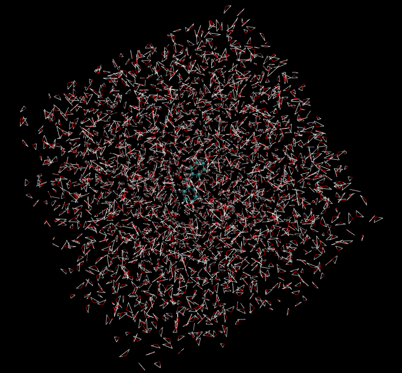
In addition to full quantum chemistry QM calculations for the system’s total energy, QM/MM calculations can be performed on molecules of interest (in this case, specifying the fifth molecule for QM calculation). The Python script for combined QM/MM energy calculation is as follows:
import glob, math, os
from pBabel import AmberCrdFile_ToCoordinates3, AmberTopologyFile_ToSystem
from pCore import logFile, Selection
from pMolecule import NBModelORCA, QCModelBDF,  System
 # Define energy calculation model
nbModel = NBModelORCA()  # Handles interactions between QM and MM regions
qcModel = QCModelBDF("GB3LYP:6-31g")
# Read system coordinates and topology information
molecule = AmberTopologyFile_ToSystem("GallicAcid.prmtop")
molecule.coordinates3 = AmberCrdFile_ToCoordinates3("GallicAcid.crd")
# Disable system symmetry
molecule.DefineSymmetry(crystalClass = None)  # QM/MM method does not support periodic boundary conditions
# Specify QM region
qm_area = Selection.FromIterable(range (72, 90))  # Specify the fifth molecule for QM calculation. (72,90) indicates atom list indices 72,73,...89 (value = atomic number -1)
# Define energy calculation model
molecule.DefineQCModel (qcModel, qcSelection = qm_area)
molecule.DefineNBModel (nbModel)
molecule.Summary()
# Calculate total energy
energy  = molecule.Energy()
The QM/MM simulation output summarizes calculation details for the MM part, QM part, and QM-MM interaction part:
----------------------------------- Summary for MM Model "AMBER" -----------------------------------
LJ 1-4 Scaling                   =          0.500  El. 1-4 Scaling                  =          0.833
Number of MM Atoms               =            288  Number of MM Atom Types          =              6
Number of Inactive MM Atoms      =             18  Total MM Charge                  =           0.00
Harmonic Bond Terms              =            288  Harmonic Bond Parameters         =              7
Harmonic Bond Inactive           =             18  Harmonic Angle Terms             =            400
Harmonic Angle Parameters        =              9  Harmonic Angle Inactive          =             25
Fourier Dihedral Terms           =            592  Fourier Dihedral Parameters      =              5
Fourier Dihedral Inactive        =             37  Fourier Improper Terms           =            112
Fourier Improper Parameters      =              1  Fourier Improper Inactive        =              7
Exclusions                       =           1216  1-4 Interactions                 =            528
LJ Parameters Form               =          AMBER  LJ Parameters Types              =              5
1-4 Lennard-Jones Form           =          AMBER  1-4 Lennard-Jones Types          =              5
----------------------------------------------------------------------------------------------------

------------------- Summary for QC Model "BDF:GB3LYP:STO-3g" -------------------
Number of QC Atoms     =             18  Boundary Atoms         =              0
Nuclear Charge         =             88  Orbital Functions      =              0
Fitting Functions      =              0  Energy Base Line       =        0.00000
--------------------------------------------------------------------------------

----------------------------- ORCA NB Model Summary ----------------------------
El. 1-4 Scaling        =       0.833333  QC/MM Coupling         =    RC Coupling
--------------------------------------------------------------------------------

------------------------------- Sequence Summary -------------------------------
Number of Atoms            =        288  Number of Components       =         16
Number of Entities         =          1  Number of Linear Polymers  =          0
Number of Links            =          0  Number of Variants         =          0
--------------------------------------------------------------------------------
Output system total energy information and contributions from each part:
--------------------------------- Summary of Energy Terms --------------------------------
Potential Energy          =    -1671893.4718  RMS Gradient              =             None
Harmonic Bond             =        1743.3211  Harmonic Angle            =         124.9878
Fourier Dihedral          =         269.8417  Fourier Improper          =           0.1346
MM/MM LJ                  =        -138.0022  MM/MM 1-4 LJ              =         474.4044
QC/MM LJ                  =         -42.2271  BDF QC                    =    -1674325.9320
------------------------------------------------------------------------------------------
QM/MM Structural Optimization
Python script for QM/MM geometry optimization:
import glob, math, os.path

from pBabel import  AmberCrdFile_ToCoordinates3, \
                    AmberTopologyFile_ToSystem , \
                    SystemGeometryTrajectory   , \
                    AmberCrdFile_FromSystem    , \
                    PDBFile_FromSystem         , \
                    XYZFile_FromSystem

from pCore import Clone, logFile, Selection

from pMolecule import NBModelORCA, QCModelBDF, System

from pMoleculeScripts import ConjugateGradientMinimize_SystemGeometry, \
                             FIREMinimize_SystemGeometry             , \
                             LBFGSMinimize_SystemGeometry            , \
                             SteepestDescentMinimize_SystemGeometry
# Define structure optimization interface
def opt_ConjugateGradientMinimize(molecule, selection):
    molecule.DefineFixedAtoms(selection)       # Fix atoms
    # Define optimization method
    ConjugateGradientMinimize_SystemGeometry(
        molecule,
        maximumIterations    =  40,   # Maximum optimization steps
        rmsGradientTolerance =  0.1, # Optimization convergence control
        trajectories   = [(trajectory, 1)]
    )   # Define trajectory save frequency
#  Define energy calculation model
nbModel = NBModelORCA()
qcModel = QCModelBDF("GB3LYP:6-31g")
# Read system coordinates and topology information
molecule = AmberTopologyFile_ToSystem ("GallicAcid.prmtop")
molecule.coordinates3 = AmberCrdFile_ToCoordinates3("GallicAcid.crd")
# Disable system symmetry
molecule.DefineSymmetry(crystalClass = None)  # QM/MM method does not support periodic boundary conditions
#. Define Atoms List
natoms = len(molecule.atoms)                      # Total number of atoms in the system
qm_list = range(72, 90)                            # QM region atoms
activate_list = range(126, 144) + range (144, 162)   # MM region active atoms (can move during optimization)
# Define MM region atoms
mm_list = range (natoms)
for i in qm_list:
    mm_list.remove(i)                              # MM region: remove QM atoms
mm_inactivate_list = mm_list[:]
for i in activate_list :
    mm_inactivate_list.remove(i)
# Input QM atoms
qmmmtest_qc = Selection.FromIterable(qm_list)
#  Define selection regions
selection_qm_mm_inactivate = Selection.FromIterable(qm_list + mm_inactivate_list)
selection_mm = Selection.FromIterable(mm_list)
selection_mm_inactivate = Selection.FromIterable(mm_inactivate_list)
# . Define the energy model.
molecule.DefineQCModel(qcModel, qcSelection = qmmmtest_qc)
molecule.DefineNBModel(nbModel)
molecule.Summary()
# Calculate total energy at optimization start
eStart = molecule.Energy()
# Define output file directory name
outlabel = 'opt_watbox_bdf'
if os.path.exists(outlabel):
    pass
else:
    os.mkdir (outlabel)
outlabel = outlabel + '/' + outlabel
# Define output trajectory
trajectory = SystemGeometryTrajectory (outlabel + ".trj" , molecule, mode = "w")
# Start first stage optimization
# Define two optimization steps
iterations = 2
#  Optimize sequentially by fixing QM and MM regions
for i in range(iterations):
    opt_ConjugateGradientMinimize(molecule, selection_qm_mm_inactivate) # Fix QM region, optimize MM
    opt_ConjugateGradientMinimize(molecule, selection_mm)                # Fix MM region, optimize QM
# Start second stage optimization
# Optimize QM and MM regions simultaneously
opt_ConjugateGradientMinimize(molecule, selection_mm_inactivate)
# Output optimized total energy
eStop = molecule.Energy()
# Save optimized coordinates (xyz/crd/pdb formats)
XYZFile_FromSystem(outlabel +  ".xyz", molecule)
AmberCrdFile_FromSystem(outlabel +  ".crd" , molecule)
PDBFile_FromSystem(outlabel +  ".pdb" , molecule)
Output system convergence information (showing first 20 steps):
----------------------------------------------------------------------------------------------------------------
Iteration       Function             RMS Gradient        Max. |Grad.|          RMS Disp.         Max. |Disp.|
----------------------------------------------------------------------------------------------------------------
 0     I   -1696839.69778731          2.46510318          9.94250232          0.00785674          0.03168860
 2   L1s   -1696839.82030342          1.38615730          5.83254788          0.00043873          0.00126431
 4   L1s   -1696839.90971371          1.41241184          5.29242524          0.00067556          0.00172485
 6   L0s   -1696840.01109863          1.41344485          4.70119338          0.00090773          0.00265969
 8   L1s   -1696840.09635696          1.44964059          5.72496661          0.00108731          0.00328490
 10  L1s   -1696840.17289698          1.28607709          4.73666387          0.00108469          0.00354577
 12  L1s   -1696840.23841524          1.03217304          3.00441004          0.00081945          0.00267931
 14  L1s   -1696840.30741088          1.40349698          5.22220965          0.00162080          0.00519590
 16  L1s   -1696840.43546466          1.32604042          4.51175225          0.00158796          0.00455431
 18  L0s   -1696840.52547251          1.27123125          4.20616166          0.00158796          0.00428040
 20  L0s   -1696840.60265453          1.08553355          3.12355616          0.00158796          0.00470223
----------------------------------------------------------------------------------------------------------------
Output system total energy information:
--------------------------------- Summary of Energy Terms --------------------------------
Potential Energy          =    -1696841.6016  RMS Gradient              =             None
Harmonic Bond             =           3.0295  Harmonic Angle            =           3.6222
Fourier Dihedral          =          32.0917  Fourier Improper          =           0.0040
MM/MM LJ                  =         -69.3255  MM/MM 1-4 LJ              =          43.9528
QC/MM LJ                  =         -47.2706  BDF QC                    =    -1696807.7057
------------------------------------------------------------------------------------------
Note
QM/MM geometry optimization is generally challenging to converge and requires advanced techniques. Common approaches include: fixing the MM region and optimizing the QM region; then fixing the QM region and optimizing the MM region. After several iterations, optimize both regions simultaneously. Convergence depends on QM region selection and whether the QM/MM boundary contains highly charged atoms. To accelerate optimization, fix the MM region and select only a suitable nearby region as the active area whose coordinates can change during optimization.
QM/MM Excited State Calculation
Based on the previous QM/MM geometry optimization, add MM region active atoms to the QM region for QM/MM-TDDFT calculations. The complete code is as follows:
import glob, math, os.path

from pBabel import  AmberCrdFile_ToCoordinates3, \
                    AmberTopologyFile_ToSystem , \
                    SystemGeometryTrajectory   , \
                    AmberCrdFile_FromSystem    , \
                    PDBFile_FromSystem         , \
                    XYZFile_FromSystem

from pCore import Clone, logFile, Selection

from pMolecule import NBModelORCA, QCModelBDF, System

from pMoleculeScripts import ConjugateGradientMinimize_SystemGeometry, \
                             FIREMinimize_SystemGeometry             , \
                             LBFGSMinimize_SystemGeometry            , \
                             SteepestDescentMinimize_SystemGeometry
# Define structure optimization interface
def opt_ConjugateGradientMinimize(molecule, selection):
    molecule.DefineFixedAtoms(selection)       # Fix atoms
    # Define optimization method
    ConjugateGradientMinimize_SystemGeometry(
        molecule,
        maximumIterations    =  40,   # Maximum optimization steps
        rmsGradientTolerance =  0.1, # Optimization convergence control
        trajectories   = [(trajectory, 1)]
    )   # Define trajectory save frequency
#  Define energy calculation model
nbModel = NBModelORCA()
qcModel = QCModelBDF("GB3LYP:6-31g")
# Read system coordinates and topology information
molecule = AmberTopologyFile_ToSystem ("GallicAcid.prmtop")
molecule.coordinates3 = AmberCrdFile_ToCoordinates3("GallicAcid.crd")
# Disable system symmetry
molecule.DefineSymmetry(crystalClass = None)  # QM/MM method does not support periodic boundary conditions
#. Define Atoms List
natoms = len(molecule.atoms)                      # Total number of atoms in the system
qm_list = range(72, 90)                            # QM region atoms
activate_list = range(126, 144) + range (144, 162)   # MM region active atoms (can move during optimization)
# Define MM region atoms
mm_list = range (natoms)
for i in qm_list:
    mm_list.remove(i)                              # MM region: remove QM atoms
mm_inactivate_list = mm_list[:]
for i in activate_list :
    mm_inactivate_list.remove(i)
# Input QM atoms
qmmmtest_qc = Selection.FromIterable(qm_list)
#  Define selection regions
selection_qm_mm_inactivate = Selection.FromIterable(qm_list + mm_inactivate_list)
selection_mm = Selection.FromIterable(mm_list)
selection_mm_inactivate = Selection.FromIterable(mm_inactivate_list)
# . Define the energy model.
molecule.DefineQCModel(qcModel, qcSelection = qmmmtest_qc)
molecule.DefineNBModel(nbModel)
molecule.Summary()
# Calculate total energy at optimization start
eStart = molecule.Energy()
# Define output file directory name
outlabel = 'opt_watbox_bdf'
if os.path.exists(outlabel):
    pass
else:
    os.mkdir (outlabel)
outlabel = outlabel + '/' + outlabel
# Define output trajectory
trajectory = SystemGeometryTrajectory (outlabel + ".trj" , molecule, mode = "w")
# Start first stage optimization
# Define two optimization steps
iterations = 2
#  Optimize sequentially by fixing QM and MM regions
for i in range(iterations):
    opt_ConjugateGradientMinimize(molecule, selection_qm_mm_inactivate) # Fix QM region, optimize MM
    opt_ConjugateGradientMinimize(molecule, selection_mm)                # Fix MM region, optimize QM
# Start second stage optimization
# Optimize QM and MM regions simultaneously
opt_ConjugateGradientMinimize(molecule, selection_mm_inactivate)
# Output optimized total energy
eStop = molecule.Energy()
# Save optimized coordinates (xyz/crd/pdb formats)
XYZFile_FromSystem(outlabel +  ".xyz", molecule)
AmberCrdFile_FromSystem(outlabel +  ".crd" , molecule)
PDBFile_FromSystem(outlabel +  ".pdb" , molecule)

#  TDDFT calculation
qcModel = QCModelBDF_template ( )
qcModel.UseTemplate (template = 'head_bdf_nosymm.inp' )

tdtest = Selection.FromIterable ( qm_list + activate_list )
# . Define the energy model.
molecule.DefineQCModel ( qcModel, qcSelection = tdtest )
molecule.DefineNBModel ( nbModel )
molecule.Summary ( )

# . Calculate
energy  = molecule.Energy ( )
Output system total energy information:
--------------------------------- Summary of Energy Terms --------------------------------
Potential Energy          =    -5088333.3818  RMS Gradient              =             None
Harmonic Bond             =           0.0000  Harmonic Angle            =           0.0000
Fourier Dihedral          =           0.0000  Fourier Improper          =           0.0000
QC/MM LJ                  =        -112.3207  BDF QC                    =    -5088221.0611
------------------------------------------------------------------------------------------
Simultaneously generate .log result files. Similar to regular excited-state calculations, information such as oscillator strength, excitation energy, and total energy of excited states can be viewed:
No.     1    w=      4.7116 eV    -1937.8276358207 a.u.  f=    0.0217   D<Pab>= 0.0000   Ova= 0.6704
  CV(0):    A( 129 )->   A( 135 )  c_i:  0.7254  Per: 52.6%  IPA:     7.721 eV  Oai: 0.6606
  CV(0):    A( 129 )->   A( 138 )  c_i:  0.2292  Per:  5.3%  IPA:     9.104 eV  Oai: 0.8139
  CV(0):    A( 132 )->   A( 135 )  c_i:  0.4722  Per: 22.3%  IPA:     7.562 eV  Oai: 0.6924
  CV(0):    A( 132 )->   A( 138 )  c_i: -0.4062  Per: 16.5%  IPA:     8.946 eV  Oai: 0.6542
Transition dipole moments are also printed:
*** Ground to excited state Transition electric dipole moments (Au) ***
 State          X           Y           Z          Osc.
    1       0.0959       0.1531       0.3937       0.0217       0.0217
    2       0.0632      -0.1286       0.3984       0.0207       0.0207
    3      -0.0797      -0.2409       0.4272       0.0287       0.0287
    4       0.0384      -0.0172      -0.0189       0.0003       0.0003
    5       1.1981       0.8618      -0.1305       0.2751       0.2751
QM/MM Case Tutorial II: Benzophenone
Benzophenone Structure Preparation
First prepare the coordinate file for benzophenone (Benzophenone), named BPH.xyz
24

C         -2.54700        0.45510        0.06680
C         -2.54160       -0.01810        1.38630
C         -3.74290       -0.40660        1.99760
C         -4.94170       -0.34290        1.28250
C         -4.94480        0.12330       -0.03620
C         -3.74920        0.52640       -0.64160
C         -1.27680       -0.08120        2.18450
O         -1.26930        0.16880        3.37250
C         -0.02150       -0.46400        1.46430
C          1.18620        0.13430        1.85330
C          2.37660       -0.21530        1.21040
C          2.36490       -1.17300        0.19100
C          1.16310       -1.78220       -0.18680
C         -0.03080       -1.42830        0.44700
H          1.18770        0.86620        2.66440
H         -3.73280       -0.75010        3.03460
H          3.31310        0.25350        1.50860
H         -5.87330       -0.64990        1.75530
H          3.29390       -1.44820       -0.30740
H         -5.88040        0.17660       -0.59220
H          1.15790       -2.53420       -0.97410
H         -3.75550        0.89780       -1.66500
H         -0.96650       -1.90720        0.15500
H         -1.61620        0.77400       -0.40440
Use Open Babel and Amber plugin antechamber to obtain bond and charge information. Command line operations:
obabel BPH.xyz -O BPH_mid.mol2
# Default molecule name is NUL; replace with BPH in mol2 file (not done in this example)
antechamber -i BPH_mid.mol2 -fi mol2 -o BPH.mol2 -fo mol2 -c bcc -at gaff
Use Amber’s parmchk tool to obtain force field parameters Command line operation:
parmchk -a Y -i BPH.mol2 -f mol2 -o BPH.frcmod
Perform solvation using tleap and obtain small molecule lib file and solvated system. Prepare tleap.in file to obtain top and crd files (named BPH_solv.top BPH_solv.crd)
source leaprc.protein.ff14SB
source leaprc.water.tip3p
loadamberparams BPH.frcmod
BPH=loadmol2 BPH.mol2
check BPH
saveoff BPH BPH.lib
solvateoct BPH TIP3PBOX 18.0
saveamberparm BPH BPH_solv.top BPH_solv.crd
quit
Command line run:
tleap -f tleap.in
Obtain initial conformation BPH_solv.top BPH_solv.crd.
Dynamics Equilibration
Create folder md/, prepare dynamics simulation files: minimization input file
01_Min.in,
heating input file
02_Heat.in,
equilibration input file
03_Prod.in.
Use Amber’s sander for molecular dynamics minimization, heating, and equilibration:
Command line sequential runs:
### Optimization
sander -O -i 01_Min.in -o 01_Min.out -p ../BPH_solv.top -c ../BPH_solv.crd -r 01_Min.rst -inf 01_Min.mdinfo
### Heat
sander -O -i 02_Heat.in -o 02_Heat.out -p ../BPH_solv.top -c 01_Min.rst -r 02_Heat.rst -x 02_Heat.mdcrd -inf 02_Heat.mdinfo
### Production
sander -O -i 03_Prod.in -o 03_Prod.out -p ../BPH_solv.top -c 02_Heat.rst -r 03_Prod.rst -x 03_Prod.mdcrd -inf 03_Prod.mdinfo
Dynamics Result Analysis
Randomly Select Single Frame Structure and Extract Partial Water Conformation
Use cpptraj to obtain single frame conformation (randomly selected for demonstration)
Prepare input file snap.trajin
parm ../BPH_solv.top
trajin 03_Prod.mdcrd 2976 2976 1      # read from mdcrd frames 2976 to 2976 (1 frame)
center :1                             # put BPH in the center
image familiar                        # re-image
trajout snapshot_2976.rst rest        # write the coordinates of this frame
go
Command line run:
cpptraj -i snap.trajin
Extract partial water conformation
Remove water molecules >20Å from C7 atom in BPH. Prepare input file strip.trajin:
parm ../BPH_solv.top
trajin snapshot_2976.rst                 # read the snapshot
reference snapshot_2976.rst rest         # use it as reference (necessary for strip command)
strip @7>:20.0                           # strip all waters further than 20A around atom C7
trajout strip_2976.pdb pdb               # write pdb output
go
Command line run:
cpptraj -i strip.trajin
Obtain new solvated system:
strip_2976.pdb.
QM/MM Calculation Preparation
Top and crd file preparation
pDynamo uses Amber’s top and crd files as input. Using strip_2976.pdb and previously generated force field files, obtain corresponding Amber top and crd files.
Create and enter folder md/get_topcrd/, prepare tleap input file
tleap.in.
source leaprc.protein.ff14SB
source leaprc.water.tip3p
loadamberparams ../../BPH.frcmod
loadoff ../../BPH.lib
a=loadpdb strip_2976.pdb
check a
saveamberparm a BPH_new.top BPH_new.crd
savepdb a BPH_new.pdb
quit
Command line run to obtain new top and crd files (
BPH_new.top,
BPH_new.crd,
BPH_new.pdb
)
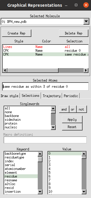
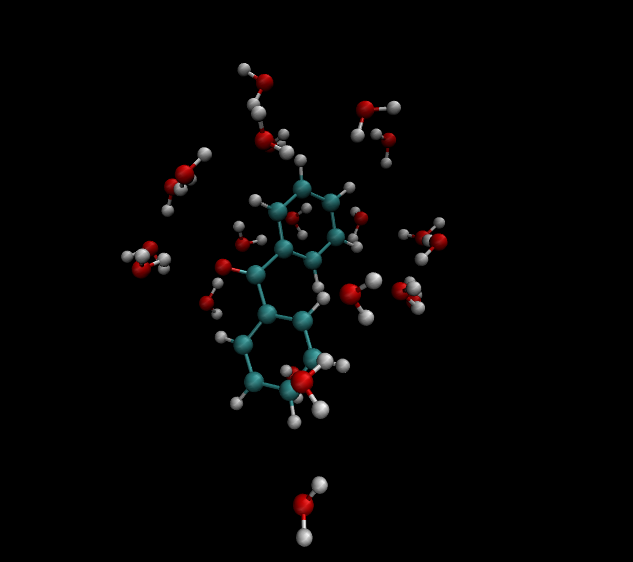
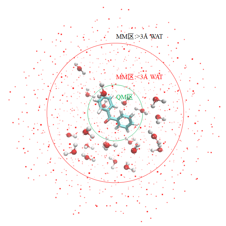
2. Active region water layer selection In VMD, select water within 3Å of benzophenone as movable water layer. Set VMD as shown below to display benzophenone and its surrounding 3Å water layer:
BPH and water within 3Å are shown below:
Overall conformation is shown below:
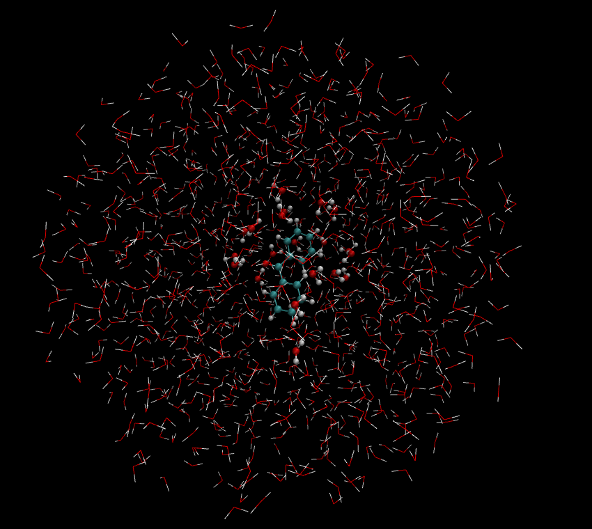
QM/MM region division for the entire system is shown below:
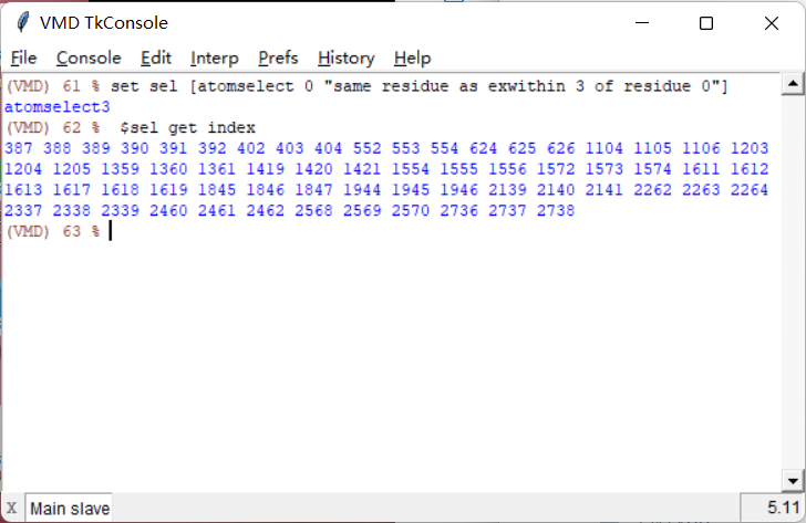
Use VMD’s TkConsole to obtain atomic indices for MM active region, which will be used in QM/MM input files. In TkConsole console, type sequentially:
As shown:
QM/MM Calculation
Ground State Optimization
Create folder qmmm/, copy BPH_new.crd and BPH_new.top to this directory
Create qmmm/ground_opt/ folder for ground state QM/MM geometry optimization
Prepare QM/MM input file opt.py, defining QM region and movable MM region:
#. Define Atoms List
natoms = len ( molecule.atoms )
qm_list = range(24)
activate_list = [387,388,389,390,391,392,402,403,404,552,553,554,624,625,626,1104,1105,1106,
                 1203,1204,1205,1359,1360,1361,1419,1420,1421,1554,1555,1556,1572,1573,1574,
                 1611,1612,1613,1617,1618,1619,1845,1846,1847,1944,1945,1946,2139,2140,2141,
                 2262,2263,2264,2337,2338,2339,2460,2461,2462,2568,2569,2570,2736,2737,2738]
mm_list = range ( natoms )
for i in qm_list :
    mm_list.remove( i )
mm_inactivate_list = mm_list[ : ]
for i in activate_list :
    mm_inactivate_list.remove( i )

# . Define the selection for the first molecule.
qmmmtest_qc = Selection.FromIterable ( qm_list )

# . Define Fixed Atoms
selection_qm_mm_inactivate = Selection.FromIterable ( qm_list + mm_inactivate_list )
Minimize for 100 steps
ConjugateGradientMinimize_SystemGeometry ( molecule                    ,
                                         logFrequency         =  2,
                                         maximumIterations    =  100,
                                         rmsGradientTolerance =  0.1,
                                         trajectories   = [ ( trajectory, 2 ) ])
QM model selection
qcModel = QCModelBDF ( "GB3LYP:6-31g" )
Full file:
opt.py
QM/MM ground state geometry optimization results
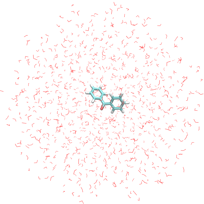
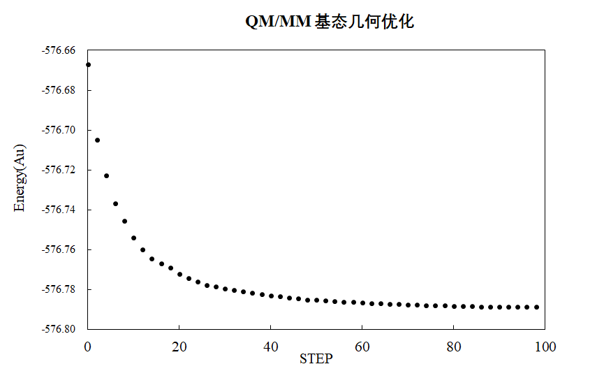
S1 State Optimization
Create qmmm/s1_opt/ folder for S1 state QM/MM geometry optimization
Prepare QM/MM input file opt.py with same QM region and movable MM region as ground state
QM model uses QCModelBDF_TDGRAD1 class with template file for excited state geometry optimization:
qcModel = qcModel = QCModelBDF_TDGRAD1 ( template = 'temple.inp', exgrad = 1 )
Full file:
opt.py;
Template file:
opt.py
sets excited state gradient to S1 state gradient.
QM/MM S1 state geometry optimization results
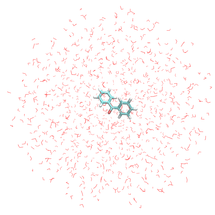
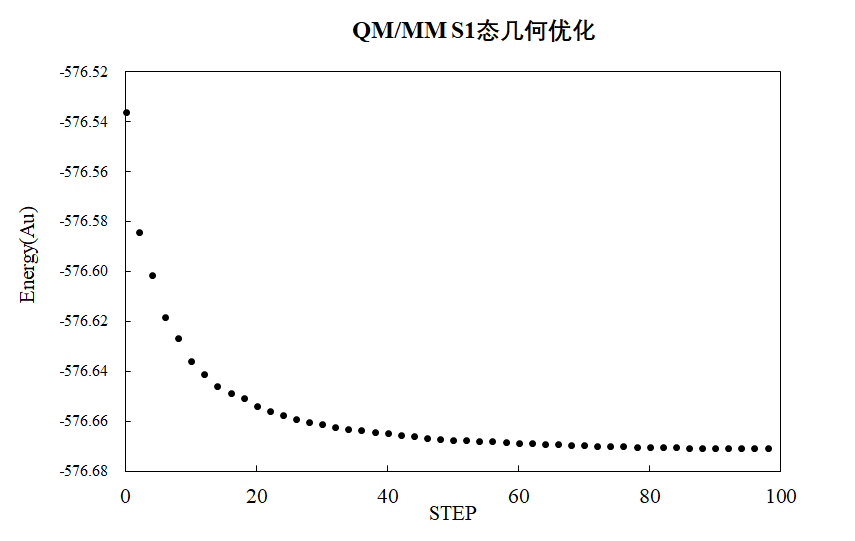
QMMM calculations for membrane protein systems
System view
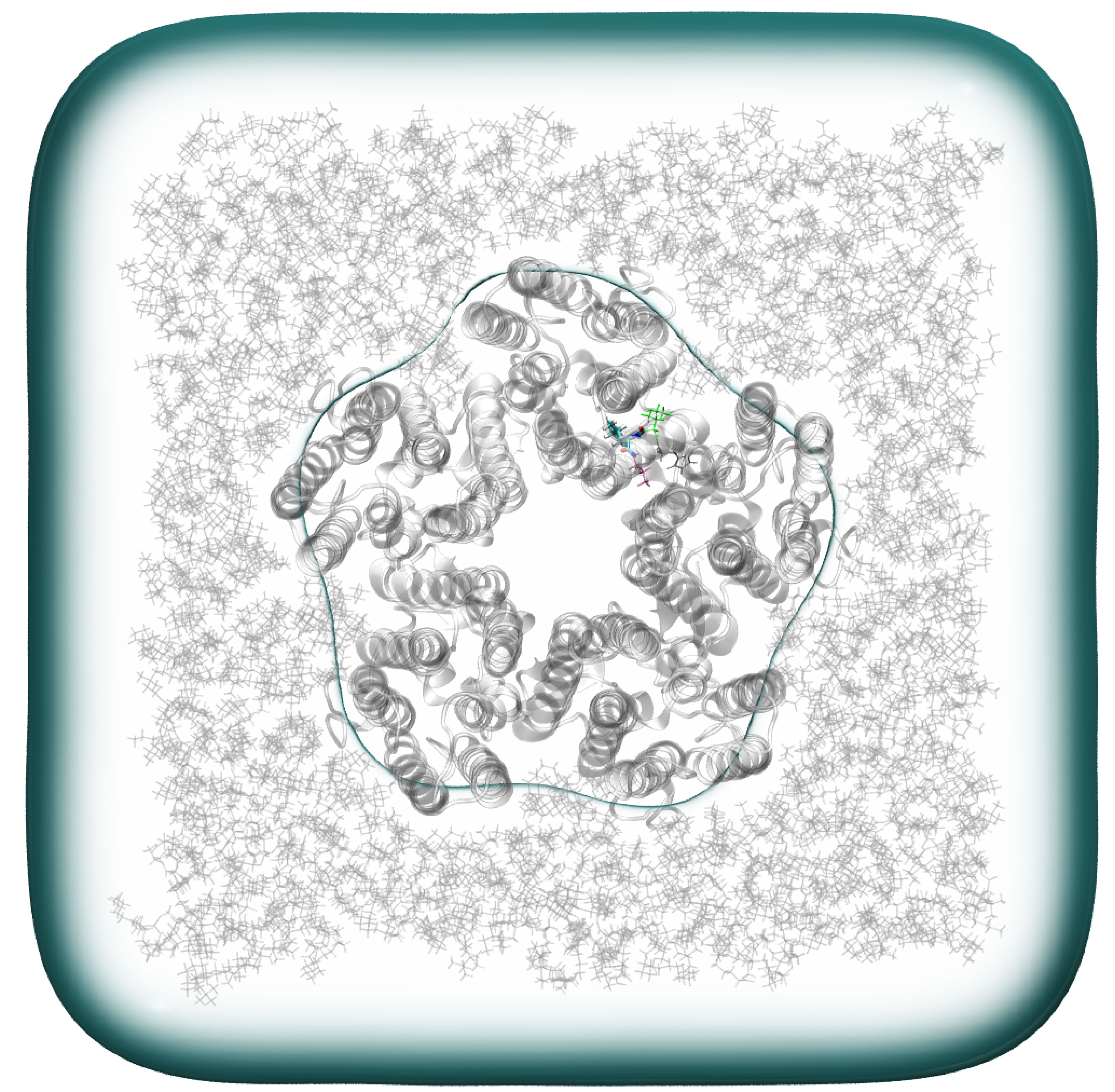
QM/MM calculation preparation
1.QM/MM input file preparation
The top file and coordinate file of the system
01_Min.in
01_Min.in
2. QM area selection LEU 30 is set as the QM region while containing adjacent C=O groups As shown in the figure, the yellowish region is the QM region atom
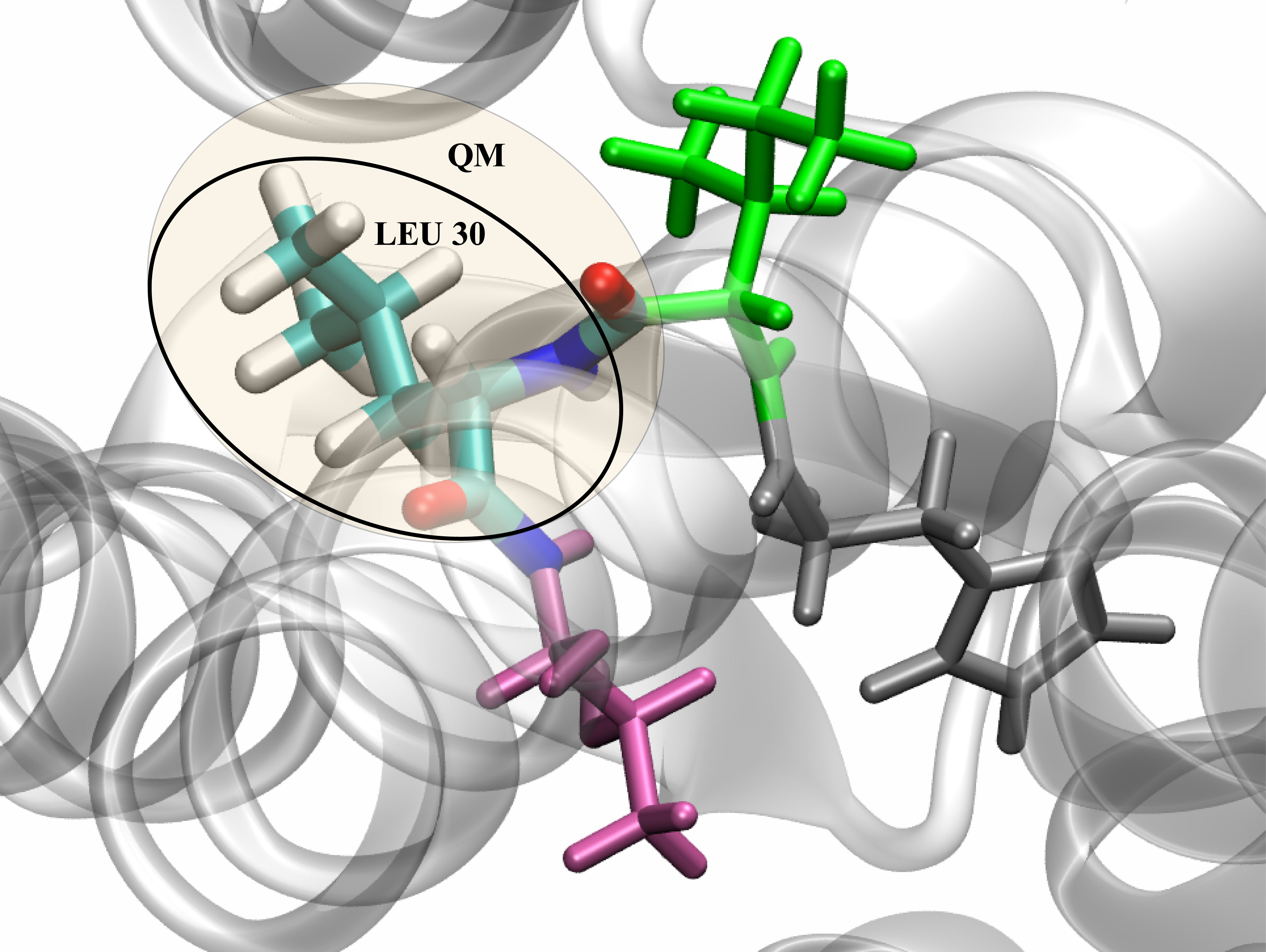
where the index of LEU 30 is:
433 434 435 436 437 438 439 440 441 442 443 444 445 446 447 448 449 450 451
The index of the C=O connection is
431 432
The index of the connected C=O is 3. MM active region molecule selection MM active region molecule selection A molecule 8Å around LEU30 was selected as the MM active region in VMD
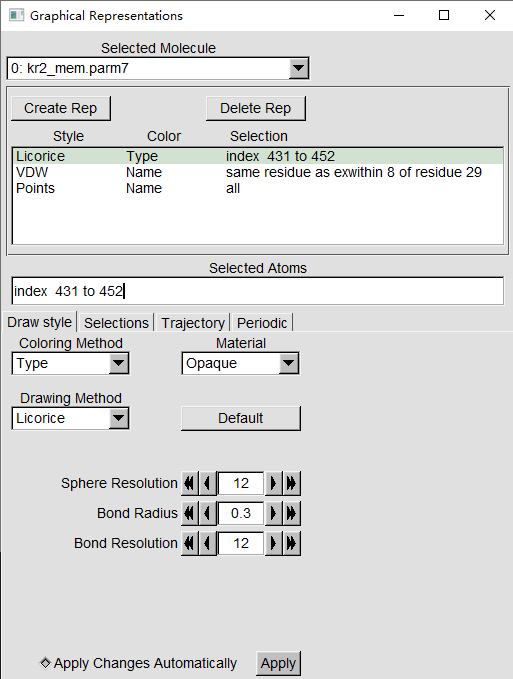
the qm/mm region contains leu30 and the surrounding 8å atoms
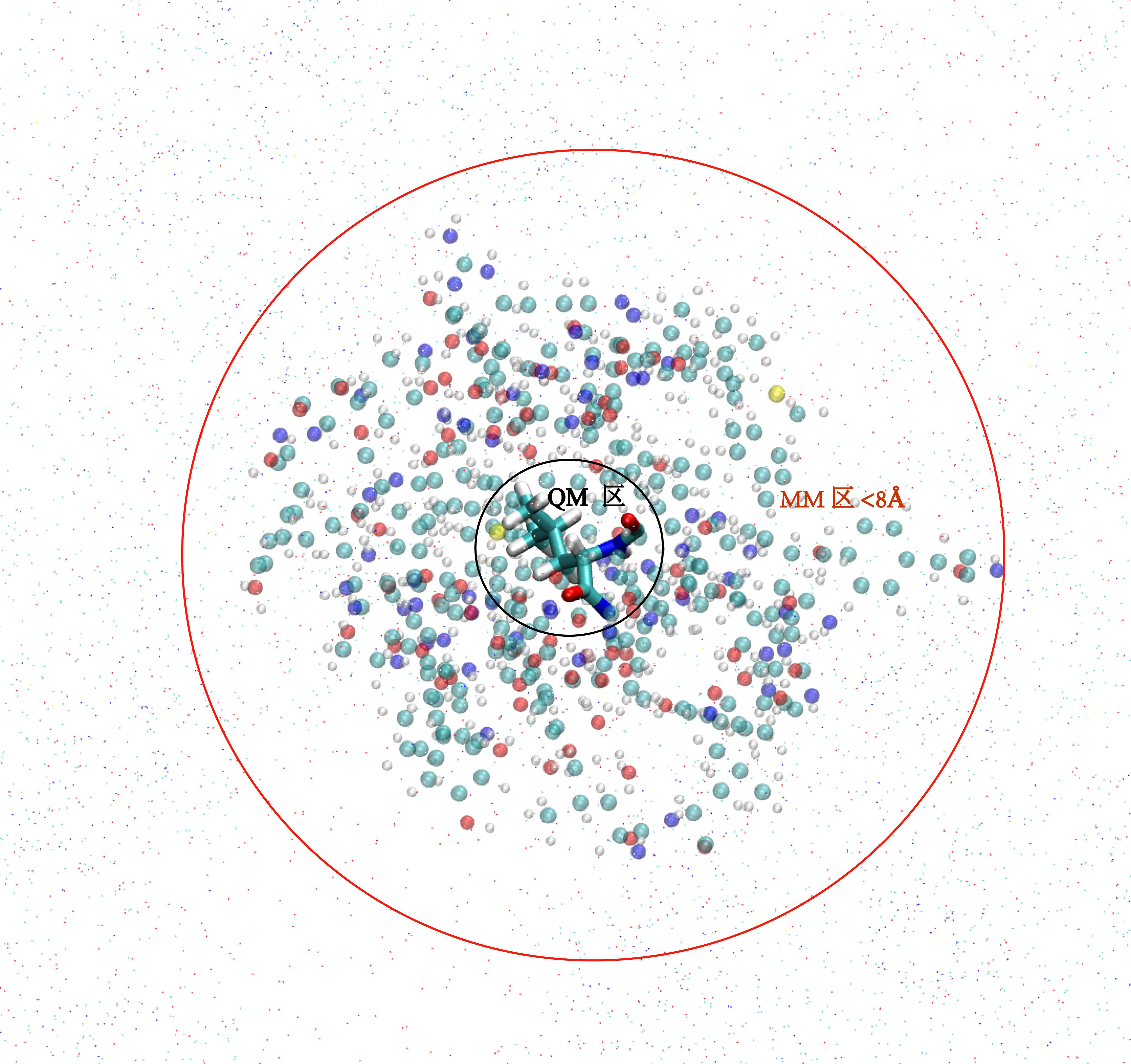
Use the TkConsole in VMD to obtain the atomic index of the active region of the MM region
In the TkConsole console, type in turn
# Choose an atom of 8Å around LEU30
set sel [atomselect 0 "same residue as exwithin 8 of residue 29"]
#Get the index of the 8Å atom around LEU30
$sel get index
As shown
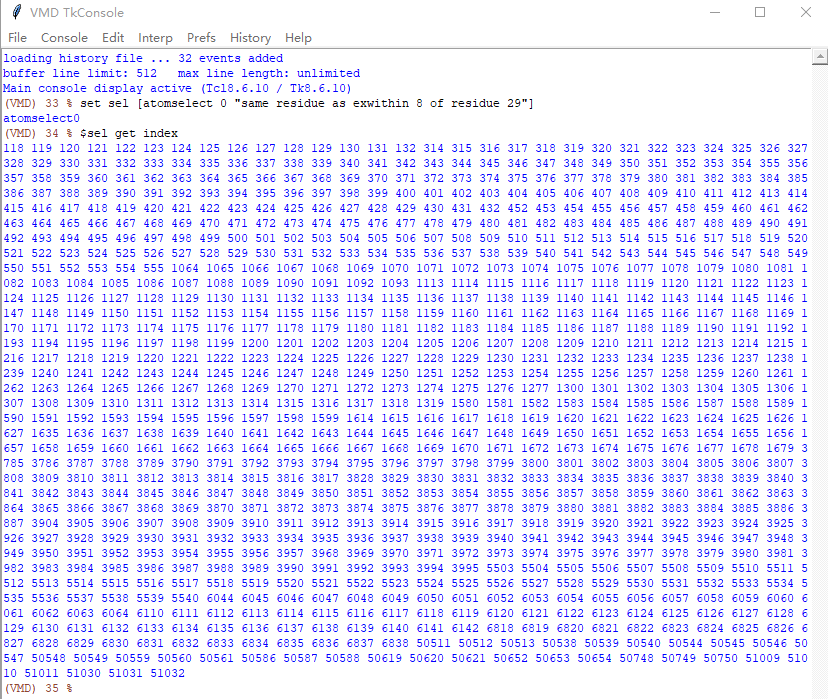
QM/MM optimization
Structural optimization
- Create a new folder qmmmopt folder to optimize the QM/MM geometry configuration of the ground state
- Prepare the QM/MM input file
opt.py
The QM area and the movable MM area are defined:
#. Define Atoms List
natoms = len ( molecule.atoms )
qm_list = range (431, 452 )
activate_list = [118,119,120,121,122,123,124,125,126,127,128,129,130,131,
                 132,314,315,316,317,318,319,320,321,322,323,324,325,326,
                 327,328,329,330,331,332,333,334,335,336,337,338,339,340,
                 341,342,343,344,345,346,347,348,349,350,351,352,353,354,
                 355,356,357,358,359,360,361,362,363,364,365,366,367,368,
                 369,370,371,372,373,374,375,376,377,378,379,380,381,382,
                 383,384,385,386,387,388,389,390,391,392,393,394,395,396,
                 397,398,399,400,401,402,403,404,405,406,407,408,409,410,
                 411,412,413,414,415,416,417,418,419,420,421,422,423,424,
                 425,426,427,428,429,430,        452,453,454,455,456,457,
                 458,459,460,461,462,463,464,465,466,467,468,469,470,471,
                 472,473,474,475,476,477,478,479,480,481,482,483,484,485,
                 486,487,488,489,490,491,492,493,494,495,496,497,498,499,
                 500,501,502,503,504,505,506,507,508,509,510,511,512,513,
                 514,515,516,517,518,519,520,521,522,523,524,525,526,527,
                 528,529,530,531,532,533,534,535,536,537,538,539,540,541,
                 542,543,544,545,546,547,548,549,550,551,552,553,554,555,
                 1064,1065,1066,1067,1068,1069,1070,1071,1072,1073,1074,1075,
                 1076,1077,1078,1079,1080,1081,1082,1083,1084,1085,1086,1087,
                 1088,1089,1090,1091,1092,1093,1113,1114,1115,1116,1117,1118,
                 1119,1120,1121,1122,1123,1124,1125,1126,1127,1128,1129,1130,
                 1131,1132,1133,1134,1135,1136,1137,1138,1139,1140,1141,1142,
                 1143,1144,1145,1146,1147,1148,1149,1150,1151,1152,1153,1154,
                 1155,1156,1157,1158,1159,1160,1161,1162,1163,1164,1165,1166,
                 1167,1168,1169,1170,1171,1172,1173,1174,1175,1176,1177,1178,
                 1179,1180,1181,1182,1183,1184,1185,1186,1187,1188,1189,1190,
                 1191,1192,1193,1194,1195,1196,1197,1198,1199,1200,1201,1202,
                 1203,1204,1205,1206,1207,1208,1209,1210,1211,1212,1213,1214,
                 1215,1216,1217,1218,1219,1220,1221,1222,1223,1224,1225,1226,
                 1227,1228,1229,1230,1231,1232,1233,1234,1235,1236,1237,1238,
                 1239,1240,1241,1242,1243,1244,1245,1246,1247,1248,1249,1250,
                 1251,1252,1253,1254,1255,1256,1257,1258,1259,1260,1261,1262,
                 1263,1264,1265,1266,1267,1268,1269,1270,1271,1272,1273,1274,
                 1275,1276,1277,1300,1301,1302,1303,1304,1305,1306,1307,1308,
                 1309,1310,1311,1312,1313,1314,1315,1316,1317,1318,1319,1580,
                 1581,1582,1583,1584,1585,1586,1587,1588,1589,1590,1591,1592,
                 1593,1594,1595,1596,1597,1598,1599,1614,1615,1616,1617,1618,
                 1619,1620,1621,1622,1623,1624,1625,1626,1627,1635,1636,1637,
                 1638,1639,1640,1641,1642,1643,1644,1645,1646,1647,1648,1649,
                 1650,1651,1652,1653,1654,1655,1656,1657,1658,1659,1660,1661,
                 1662,1663,1664,1665,1666,1667,1668,1669,1670,1671,1672,1673,
                 1674,1675,1676,1677,1678,1679,3785,3786,3787,3788,3789,3790,
                 3791,3792,3793,3794,3795,3796,3797,3798,3799,3800,3801,3802,
                 3803,3804,3805,3806,3807,3808,3809,3810,3811,3812,3813,3814,
                 3815,3816,3817,3828,3829,3830,3831,3832,3833,3834,3835,3836,
                 3837,3838,3839,3840,3841,3842,3843,3844,3845,3846,3847,3848,
                 3849,3850,3851,3852,3853,3854,3855,3856,3857,3858,3859,3860,
                 3861,3862,3863,3864,3865,3866,3867,3868,3869,3870,3871,3872,
                 3873,3874,3875,3876,3877,3878,3879,3880,3881,3882,3883,3884,
                 3885,3886,3887,3904,3905,3906,3907,3908,3909,3910,3911,3912,
                 3913,3914,3915,3916,3917,3918,3919,3920,3921,3922,3923,3924,
                 3925,3926,3927,3928,3929,3930,3931,3932,3933,3934,3935,3936,
                 3937,3938,3939,3940,3941,3942,3943,3944,3945,3946,3947,3948,
                 3949,3950,3951,3952,3953,3954,3955,3956,3957,3968,3969,3970,
                 3971,3972,3973,3974,3975,3976,3977,3978,3979,3980,3981,3982,
                 3983,3984,3985,3986,3987,3988,3989,3990,3991,3992,3993,3994,
                 3995,5503,5504,5505,5506,5507,5508,5509,5510,5511,5512,5513,
                 5514,5515,5516,5517,5518,5519,5520,5521,5522,5523,5524,5525,
                 5526,5527,5528,5529,5530,5531,5532,5533,5534,5535,5536,5537,
                 5538,5539,5540,6044,6045,6046,6047,6048,6049,6050,6051,6052,
                 6053,6054,6055,6056,6057,6058,6059,6060,6061,6062,6063,6064,
                 6110,6111,6112,6113,6114,6115,6116,6117,6118,6119,6120,6121,
                 6122,6123,6124,6125,6126,6127,6128,6129,6130,6131,6132,6133,
                 6134,6135,6136,6137,6138,6139,6140,6141,6142,6818,6819,6820,
                 6821,6822,6823,6824,6825,6826,6827,6828,6829,6830,6831,6832,
                 6833,6834,6835,6836,6837,6838,50511,50512,50513,50538,50539,
                 50540,50544,50545,50546,50547,50548,50549,50559,50560,50561,
                 50586,50587,50588,50619,50620,50621,50652,50653,50654,50748,
                 50749,50750,51009,51010,51011,51030,51031,51032]
mm_list = range ( natoms )
for i in qm_list :
    mm_list.remove( i )
mm_inactivate_list = mm_list[ : ]
for i in activate_list :
    mm_inactivate_list.remove( i )

# . Define the selection for the first molecule.
qmmmtest_qc = Selection.FromIterable ( qm_list )

# . Define Fixed Atoms
selection_qm_mm_inactivate = Selection.FromIterable ( qm_list + mm_inactivate_list )
selection_mm = Selection.FromIterable ( mm_list )
selection_mm_inactivate = Selection.FromIterable ( mm_inactivate_list )
Iteratively optimize the MM area and QM area
# . Optimization.
# . Define the number of iterations
iterations = 2
# . QM region and MM region were fixed in turn for optimization
for i in range ( iterations ):
    opt_LBFGSMinimize ( molecule, selection_qm_mm_inactivate )
    opt_LBFGSMinimize ( molecule, selection_mm)
# . QM region and MM region were optimized simultaneously
opt_LBFGSMinimize ( molecule, selection_mm_inactivate)
QM Model Selection NB Model Selection
# . Define the energy models.
nbModel = NBModelBDF ( )
nbModel.SetOptions (qcmmCoupling = 'Z1 Coupling')
qcModel = QCModelBDF ( "GB3LYP:6-31g" )
Optimize the structure and the original structural configuration
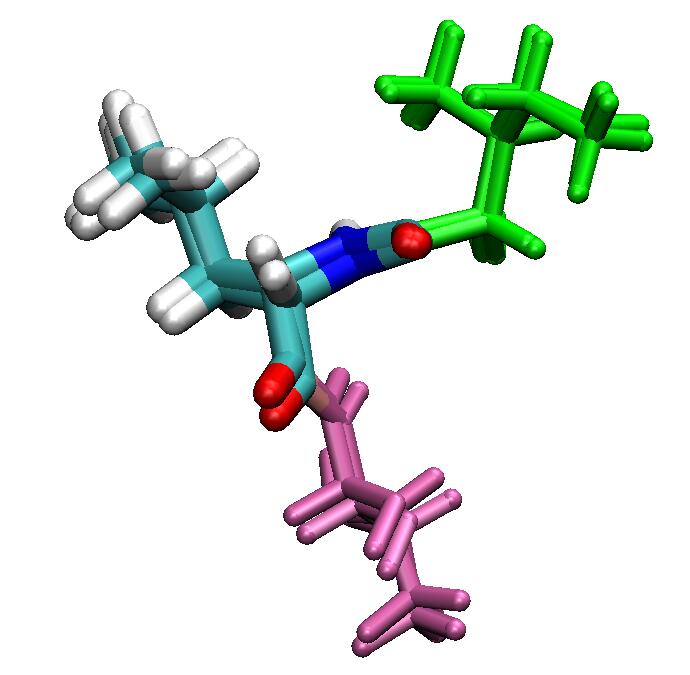
QM/MM Boundary Selection Example Tutorial
This tutorial demonstrates how QM/MM boundary selection affects geometry optimization. Incorrect boundary selection may lead to unexpected conformational changes.
System View
This example uses a pentapeptide as the computational system to test QM region selection. The system
(5ala.pdb)
consists of five ALAs, with N-terminus and C-terminus capped with ACE and NME respectively.
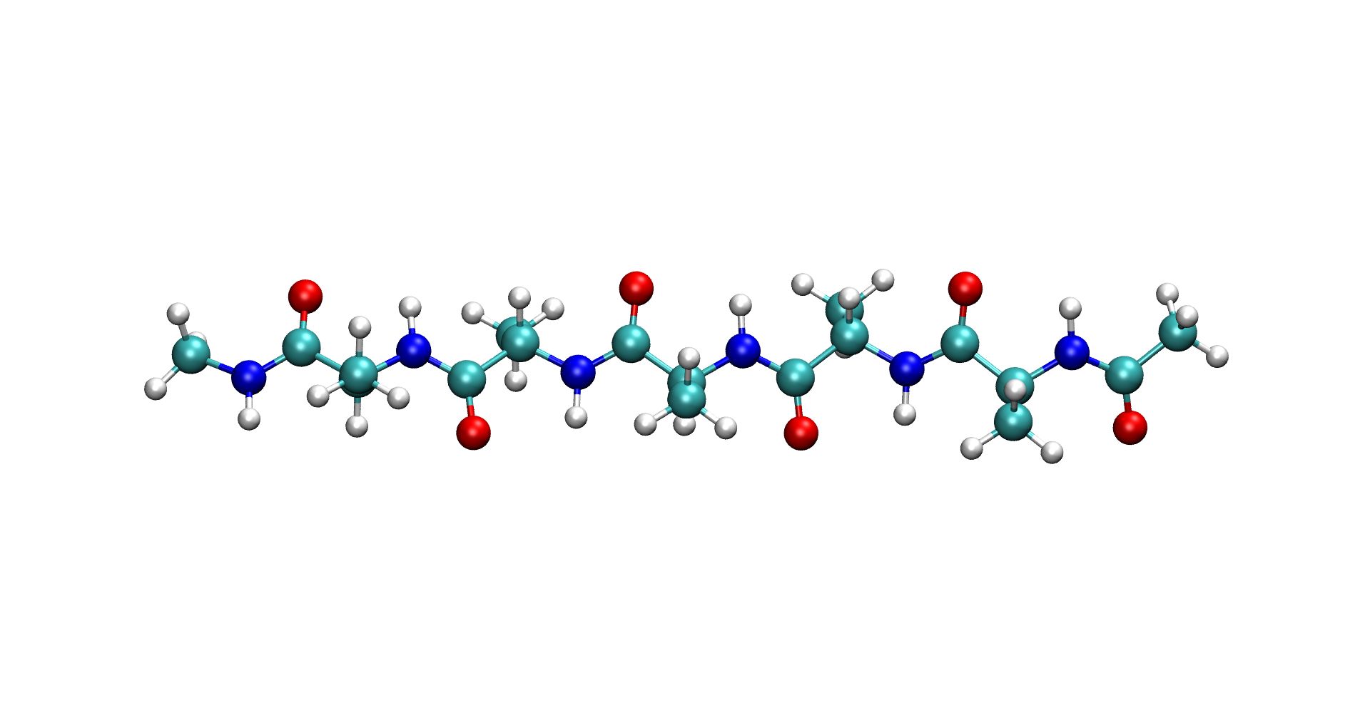
QM Region Selection
Using pentapeptide system as example:
QM Region Selection 1:
Select third alanine ALA4 as QM region, adjacent ALAs as active MM region
qm_list = range (26, 36 )
activate_list = range ( 16, 26 ) + range ( 36, 46 )
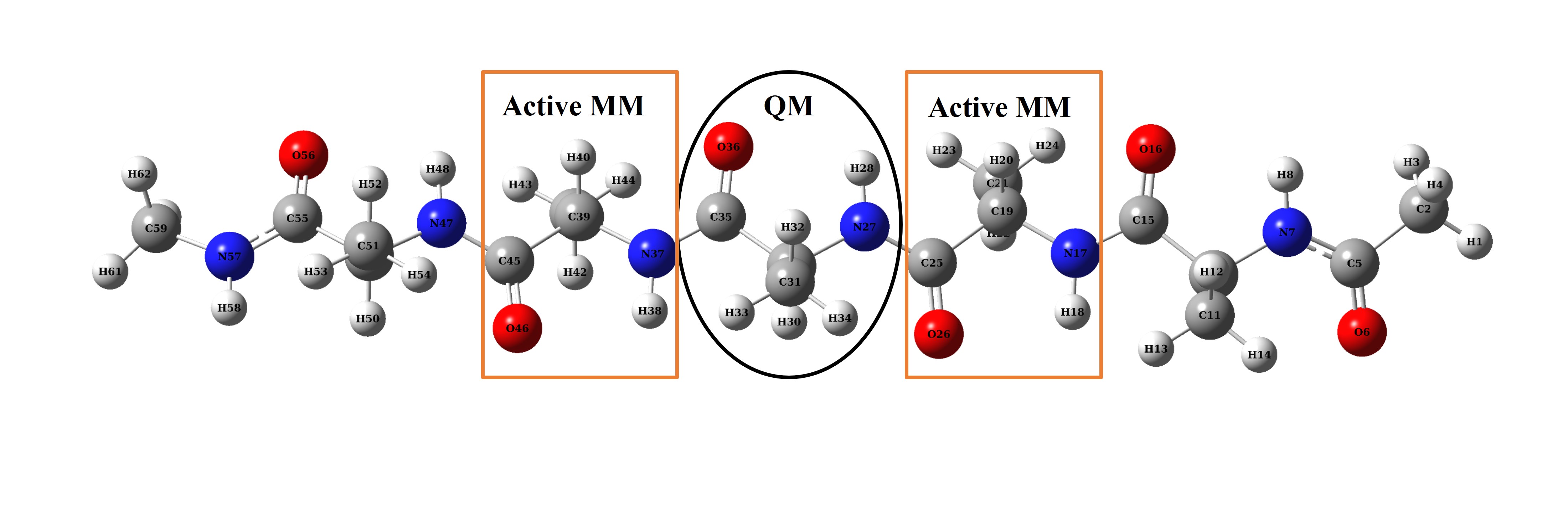
QM/MM Optimization Result
When selecting QM region, if adjacent MM region carries strong charges (e.g., C=O in this case), strong electrostatic interactions between QM and MM regions prevent system convergence. As shown in animation, large charges in adjacent MM region cause issues in QM region structure optimization.
QM Region Selection 2:
Select third alanine ALA4 as QM region plus adjacent C=O group, with other adjacent ALAs as active MM region
qm_list = range (24, 36 )
activate_list = range ( 16, 24 ) + range ( 36, 46 )
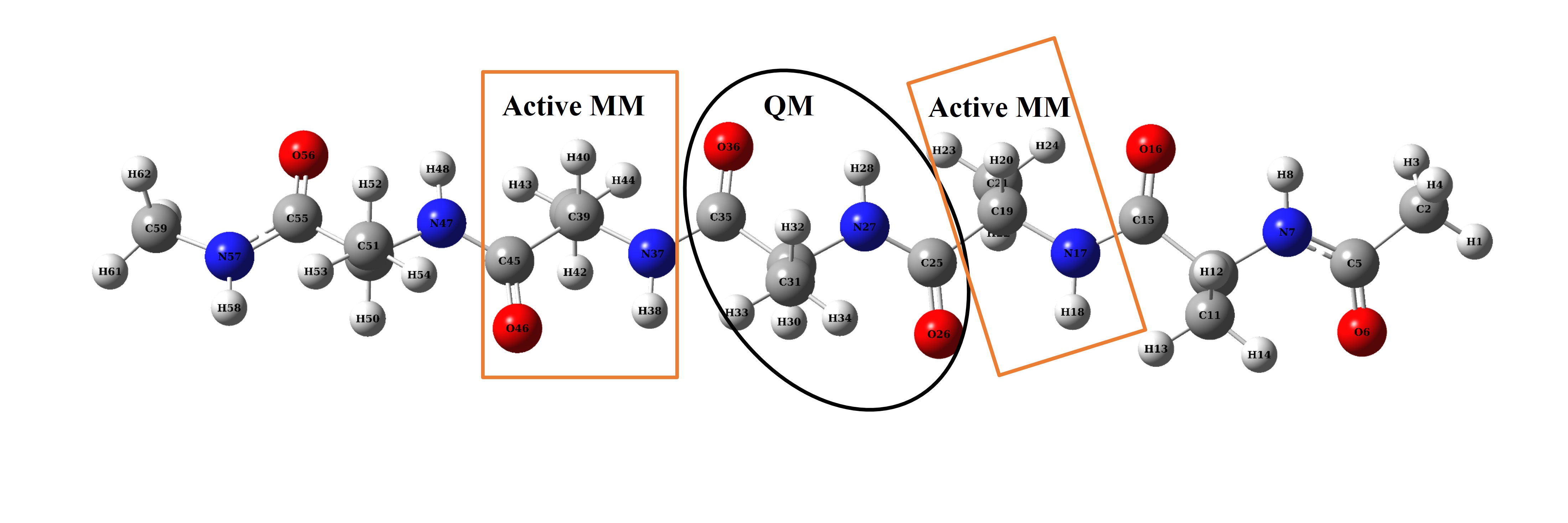
QM/MM Optimization Result
Including C=O group in QM region enables system convergence, with structure optimizing within reasonable range.
Photophysical characterization of blue light HLCT molecules
Photophysical characterization of blue light HLCT molecules
Organic light-emitting diodes (OLEDs) are widely used in display and lighting, among which light-emitting dyes are the most critical part of OLED devices. When holes and electrons recombine in the light-emitting layer, the luminescent dye molecule is excited to the excited state (Figure 1a). According to exciton statistical rules, this recombination produces 25% singlet excitons and 75% triplet excitons. According to the selection rule, 75% of the triplet excitons are wasted because the triplet to singlet transition of a pure organic system is usually forbidden. Utilizing triplet excitons through appropriate methods is a challenge for the design of OLED luminescent dye molecules.
The hybrid local-charge transfer excited state (HLCT) proposed by Ma Yuguang’s group is a luminescence mechanism that can use triplet excitons. By constructing the excited state of :math:’rm S_{1}’ with HLCT characteristics, the orbital coupling of :math:’rm T_{n}’ - :math:’rm S_{1}’ can be increased (El-Sayed rule) to facilitate the anti-system crossing (RISC) of :math:’rm T_{n}’ - :math:’rm S_{1}’. In addition, increasing the energy level difference of :math:’rm T_{n}’ - :math:’rm T_{1}’ and decreasing the energy level difference of :math:’rm T_{n}’ - :math:’rm S_{1}’ is also beneficial for the anti-system crossing. Linking the donor to the aromatic ring is a common method for constructing HLCT molecules.
Due to the higher energy levels, the photostability of blue light HLCT molecules is generally poor. Py is a class of aromatic rings with high light stability, while diphenylamine (TPA) is a common strong donor fragment. Linking the two with a single bond may be a means of constructing a highly stable blue-light HLCT molecule (Fig. 1b). In this paper, we will investigate whether 4,9-dimethyl-1-N,1-N,6-N,6-N-tetraphenylpyrene-1,6-diamine (2TPA-Py) has the characteristics of blue light HLCT by quantum chemical calculations, and verify the feasibility of the molecular design of donor-π-donor.
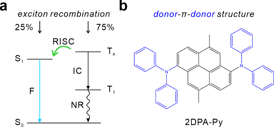
Figure 1. (a) Schematic diagram of the electroluminescence mechanism of the HLCT molecule. (b) Molecular structure of 2DPA-Py.
Ground state :math:’rm S_{0}’
Before we can make accurate calculations on the molecule, we need to obtain a reliable ground state structure ( :math:’rm S_{0}’ ), that is, structural optimization and vibration analysis of the ground state. Firstly, Gaussian was used to optimize the structure of the ground state of the molecule: math:’rm S_{0}’, using the functional B3LYP, the basis group 6-31g**, and considering the dispersion correction. The B3LYP functional was chosen because of its high computational efficiency, low dependence on the accuracy of the integration lattice, and DFT-D3(BJ) dispersion correction to describe possible non-covalent bonding interactions. In addition, because the calculation results are less sensitive to the base set for structural optimization and vibration analysis, the selection of a small base group can save time. The gjf input file is as follows: .. code-block:: bdf
%nprocshared=32 %chk=opt.chk #P B3LYP/6-31g** em=GD3BJ opt freq
Title Card Required
0 1 C 1.23142086399057 -0.01598991339220 -0.21183114910141 C 2.72871444990389 -0.00550853390551 -0.13727964385924 C 3.41061821385248 -1.20117932087473 -0.03319288637410 C 4.79904649004982 -1.26160428059098 0.03464278981730 N 5.41364048996203 -2.51932450120475 0.15418467741142 C 4.92747565422558 -3.57250001859245 -0.62664098365207 C 4.55022212480360 -3.33536995952102 -1.94901522652513 C 4.05642159683765 -4.36315245643423 -2.72763628208729 C 3.93617240694700 -5.64193595032452 -2.20823626842045 C 4.30884346659409 -5.88288539461667 -0.89597870946301 C 4.79580537663213 -4.85982627352166 -0.10603578378833 C 6.36147678282021 -2.74991702364612 1.15337779307768 C 6.31970072442968 -2.03371232006357 2.35000679508950 C 7.27393251117782 -2.25099389609825 3.32426315813784 C 8.27590697003017 -3.18766118708190 3.13164605217437 C 8.32033728954936 -3.90430287118972 1.94668478315316 C 7.37766488670707 -3.68777915010114 0.96152123805281 C 5.55426311556430 -0.07485171406329 -0.01954737716259 C 4.87062379765459 1.16805677077445 -0.07171305294141 C 3.45350429641720 1.20058735786973 -0.14489187126324 C 2.81032456952191 2.46548965694624 -0.24263234170365 C 3.51112662376826 3.62218562784879 -0.20116625218499 C 4.92681570379474 3.62501895614023 -0.06751464021658 C 5.61185537735068 2.38194680680533 -0.05584863189100 C 7.03069025627284 2.34956069156028 -0.03333330974132 C 7.67833561978987 1.08357530517932 -0.06820637808522 C 6.97580495150633 -0.07284382674662 -0.05720475575518 C 7.75357292329654 3.55630546250584 0.00437058511537 C 7.06657662311645 4.75304774446334 0.04578195006735 C 5.67683694346796 4.81291513479720 0.02109801284253 N 5.05364278941578 6.07063412409978 0.08634601203580 C 4.04430276290905 6.30650817126718 1.02225220987505 C 4.01813497397634 5.60452422886364 2.22773071875455 C 3.00342478983393 5.82342539394774 3.13839692752355 C 2.00692660848240 6.74799998492145 2.87285054139819 C 2.02998237520816 7.45096162278722 1.67912787314289 C 3.03391132115340 7.23257419582758 0.75684192709414 C 5.58014732987927 7.11518216961340 -0.67889062460768 C 6.04635677519681 6.86001855649965 -1.96924843092115 C 6.57901675320538 7.88011253315299 -2.73218118328052 C 6.65054552833193 9.16913005476952 -2.22939545341485 C 6.19012117760983 9.42795662197789 -0.94876996878721 C 5.66385569959879 8.41283112869426 -0.17399231367271 C 9.25252702611257 3.56676709389692 0.02982018386394 H 0.85832992156275 -1.03632876280351 -0.16904659946900 H 0.88933685332284 0.43501238502809 -1.14286926646989 H 0.79789574594339 0.54473304731639 0.61552131117326 H 2.85548199101679 -2.12853502172196 0.00413662861935 H 4.64873169324299 -2.33946969900849 -2.35587693447180 H 3.76953281079583 -4.16566889381519 -3.75015021922513 H 3.55256748783067 -6.44401899690169 -2.82037387929308 H 4.20934558011874 -6.87446192152345 -0.47900026581524 H 5.06879641140089 -5.04938936946588 0.92181407561931 H 5.53591434202605 -1.30746574426274 2.50753626302272 H 7.22917194113817 -1.68928048139264 4.24582973230498 H 9.01732005764785 -3.35753750290448 3.89755908403090 H 9.10183011620465 -4.63207070344374 1.78327798868360 H 7.42600935609078 -4.23604224027954 0.03176328355712 H 1.73842332597976 2.49952836140925 -0.35594215471611 H 2.99326193531308 4.56447070267168 -0.28988821662774 H 8.75546098773894 1.04836100119705 -0.10774432599440 H 7.49820003451026 -1.01601354833581 -0.09649295442825 H 7.61798445128552 5.68140497373268 0.10650429470265 H 4.79705375266048 4.88765786929865 2.44212003924378 H 2.99594325952520 5.27247674972545 4.06748299539966 H 1.21761156723492 6.91895418257396 3.58905207574990 H 1.25350653787419 8.16906880804979 1.45894118248852 H 3.03809992945878 7.76959529262987 -0.18069135423844 H 5.98545198075639 5.85630503175884 -2.36409915773676 H 6.93473355133126 7.66838923944818 -3.72993019870071 H 7.06415340233785 9.96525107867144 -2.82966866197266 H 6.25071932363493 10.42779312892758 -0.54419248783976 H 5.32231798384009 8.61698483651345 0.83028525237055 H 9.62929685852355 3.02395636423240 0.89604599037109 H 9.62231936463369 4.58813097786218 0.07624892230056 H 9.65623043406863 3.09668205158134 -0.86638315237225
Gaussian uses four criteria to determine whether the molecular structure is convergent based on four criteria: Force-RMS, Force-Max, Step-RMS, and Step-Max. After the job is finished, open the log output file and find the following keywords
         Item               Value     Threshold  Converged?
Maximum Force            0.000012     0.000450     YES
RMS     Force            0.000002     0.000300     YES
Maximum Displacement     0.001298     0.001800     YES
RMS     Displacement     0.000336     0.001200     YES
Predicted change in Energy=-5.865194D-09
Optimization completed.
   -- Stationary point found.
The convergent structure is extracted as the initial structure for subsequent calculations. The following screenshot is a partial capture:
                            Standard orientation:
---------------------------------------------------------------------
Center     Atomic      Atomic             Coordinates (Angstroms)
Number     Number       Type             X           Y           Z
---------------------------------------------------------------------
     1          6           0        1.565649   -4.134284   -0.176953
     2          6           0        1.643599   -2.628388   -0.152751
     3          6           0        2.886000   -2.003080   -0.112539
     4          6           0        3.020859   -0.613479   -0.088550
     5          7           0        4.325420   -0.044576   -0.036499
     6          6           0        5.278240   -0.466495   -0.995386
     7          6           0        4.884618   -0.626003   -2.332720
When the molecule is at the smallest point of the potential energy plane, there is generally no imaginary frequency (negative frequency). In order to verify the reliability of the structure, the frequency calculations are also checked. In the ‘log’’ output file, find the following keywords, since the vibrational frequencies are arranged from small to large, observing that the first few frequencies have no imaginary frequency, indicating that the molecule is at the local minimum point of the potential energy surface, and its molecular structure is generally reliable.
                     1                      2                      3
                     A                      A                      A
Frequencies --     12.2419                16.5051                20.1875
Red. masses --      5.7419                 5.7737                 5.1174
Frc consts  --      0.0005                 0.0009                 0.0012
IR Inten    --      0.0197                 0.0135                 1.5193
 Atom  AN      X      Y      Z        X      Y      Z        X      Y      Z
    1   6     0.01   0.00  -0.04    -0.01  -0.00  -0.09    -0.02   0.03  -0.18
    2   6     0.00   0.00  -0.04    -0.01  -0.01  -0.07    -0.02   0.03  -0.12
    3   6     0.00   0.00  -0.03    -0.01  -0.01  -0.06    -0.02   0.03  -0.11
    4   6     0.00   0.00  -0.03    -0.00  -0.01  -0.04    -0.01   0.03  -0.06
    5   7    -0.00   0.01  -0.01    -0.01  -0.01  -0.00    -0.01   0.02  -0.05
absorption spectrum
The ground state of most organic molecules is a closed shell, usually a singlet state, which is generally denoted by :math:’rm S_{0}’. According to the first law of photochemistry (Stark-Einstein), a molecule needs to absorb a photon to make a single electron jump from an occupied orbital to an unoccupied orbital, and the energy of that photon must be consistent with the energy difference between the ground state and the excited state.
So as long as a molecule is irradiated with light of the right energy, will it absorb photons to reach the excited state of electrons?
In quantum mechanics, it can be deduced from Fermi’s Golden Rule that a molecule needs to meet multiple conditions to transition from one state to another, which is called the selection rule. The specific derivation process will not be described here, but it is recommended that readers directly consult the relevant books on optical physics, and here is a brief list of some of the selection rules applicable to pure organic systems:
Satisfies the Franck-Condon principle, which states that the geometry (nucleus position) of the initial and final state molecules does not change during the electron transition.
If the geometry of the excited state is very different from the ground state, then the geometry of the molecule needs to change when the electron is excited from the lowest vibrational energy level of the ground state to the lowest vibrational energy level of the excited state. However, since the mass of the nucleus is much larger than that of the electrons and cannot keep up with the speed of the electrons, the probability of such excitation is small.
The electron spin does not change
Under the single-electron approximation, the spin orbit is orthogonally normalized. If the spins before and after the transition are different, the spin overlap integral must be 0, i.e., the transition prohibition. This is the spin selection rule: “Singlet → singlet, triplet→ triplet are allowed; Singlet →triplet, triplet →singlet forbidden”.
Track overlap
There must be overlap of the molecular orbitals before and after the transition, otherwise the dipole moment integral of the electronic transition is 0, that is, the transition is forbidden.
Orbital symmetry changes
If the molecular orbitals are symmetrical, the orbital symmetry before and after the transition must be different except for the overlapping orbitals. According to the center inversion symmetry, the orbit is divided into g (center symmetry) and u (center antisymmetry), and the specific statement is: “g→u, u→g allowed, u →u, g → g forbidden”.
It is often customary to describe the electron transition problem in the form of a transition from an orbital electron to a virtual orbital, such as natural transition orbital (NTO) analysis: the nature of the transition is illustrated by a pair of dominant orbital transition patterns. For the analysis of the electronic structure of the excited state, the time-dependent density functional (TDDFT) calculation is required, and in this case, the excited state selects the M062x functional and the Def2SVP basis group, and calculates 8 states for the singlet state and triplet state, respectively. The choice of the M062x functional is to speculate that the ground state of the molecule may have partial charge transfer (CT) properties. For this class of excited states, if you choose a functional with a lower HF component, A ghost state (a state that does not exist) may occur. To be on the safe side, choose M062x with a high HF content. Of course, functionals of other HF components such as CAM-B3LYP and ωB97XD can also be used. The key word IOP(9/40=4)’’ is to output more orbital information, so that the pair of NTOs that contribute the most to the electron excitation can be found after the MO is transformed into NTO. The gjf input file is as follows:
%nprocshared=32
%mem=6GB
%chk=tddft.chk
#P M062x/Def2SVP TD(nstates=8, 50-50) IOP(9/40=4)

Title Card Required

0 1
 C                  1.565649   -4.134284   -0.176953
 C                  1.643599   -2.628388   -0.152751
 C                  2.886000   -2.003080   -0.112539
 C                  3.020859   -0.613479   -0.088550
 N                  4.325420   -0.044576   -0.036499
 C                  5.278240   -0.466495   -0.995386
 C                  4.884618   -0.626003   -2.332720
 C                  5.799622   -1.064339   -3.285338
 C                  7.121820   -1.335486   -2.928150
 C                  7.515238   -1.172730   -1.598991
 C                  6.603320   -0.752040   -0.633991
 C                  4.698175    0.744156    1.076980
 C                  4.091832    0.542012    2.325047
 C                  4.427797    1.352319    3.406784
 C                  5.379893    2.362883    3.271786
 C                  5.988191    2.561344    2.030562
 C                  5.647767    1.769732    0.937881
 C                  1.876752    0.211899   -0.120738
 C                  0.588755   -0.407573   -0.126231
 C                  0.473733   -1.832327   -0.148612
 C                 -0.837555   -2.410247   -0.178205
 C                 -1.959943   -1.640762   -0.161854
 C                 -1.876694   -0.212016   -0.120592
 C                 -0.588696    0.407452   -0.126517
 C                 -0.473668    1.832190   -0.149905
 C                  0.837623    2.410088   -0.179888
 C                  1.960009    1.640614   -0.162984
 C                 -1.643530    2.628249   -0.154622
 C                 -2.885933    2.002973   -0.113981
 C                 -3.020804    0.613392   -0.088992
 N                 -4.325380    0.044559   -0.036541
 C                 -4.698230   -0.743314    1.077511
 C                 -4.091928   -0.540291    2.325457
 C                 -4.428022   -1.349755    3.407783
 C                 -5.380213   -2.360326    3.273499
 C                 -5.988485   -2.559645    2.032401
 C                 -5.647934   -1.768883    0.939143
 C                 -5.278162    0.465750   -0.995788
 C                 -4.884527    0.624147   -2.333249
 C                 -5.799513    1.061738   -3.286228
 C                 -7.121702    1.333222   -2.929264
 C                 -7.515137    1.171550   -1.599978
 C                 -6.603236    0.751616   -0.634632
 C                 -1.565577    4.134127   -0.179894
 H                  2.565826   -4.573123   -0.163055
 H                  1.054624   -4.497512   -1.075888
 H                  1.015461   -4.526102    0.685940
 H                  3.789152   -2.604760   -0.095814
 H                  3.860188   -0.404796   -2.611283
 H                  5.478783   -1.182339   -4.316028
 H                  7.834889   -1.669709   -3.674725
 H                  8.537506   -1.389762   -1.303667
 H                  6.910123   -0.642734    0.399820
 H                  3.355698   -0.245579    2.436971
 H                  3.946094    1.182749    4.365139
 H                  5.642450    2.988231    4.118776
 H                  6.724707    3.349483    1.905053
 H                  6.110094    1.939850   -0.027830
 H                 -0.934317   -3.489037   -0.217496
 H                 -2.937842   -2.104213   -0.185630
 H                  0.934386    3.488850   -0.219935
 H                  2.937915    2.104041   -0.187063
 H                 -3.789080    2.604673   -0.097685
 H                 -3.355727    0.247315    2.436831
 H                 -3.946346   -1.179515    4.366033
 H                 -5.642871   -2.985014    4.120945
 H                 -6.725084   -3.347795    1.907449
 H                 -6.110250   -1.939666   -0.026456
 H                 -3.860104    0.402673   -2.611627
 H                 -5.478667    1.178888   -4.317013
 H                 -7.834757    1.666861   -3.676114
 H                 -8.537402    1.388848   -1.304838
 H                 -6.910046    0.643140    0.399265
 H                 -1.015334    4.526556    0.682686
 H                 -2.565752    4.572979   -0.166245
 H                 -1.054607    4.496714   -1.079120
After the job is completed, the energy level of the low excited state is plotted according to the excited energy. It can be seen that the energy level difference between the :math:’rm S_{1}’ state and the :math:’rm T_{2}’ and :math:’rm T_{3}’ states is small, and if the rotary-orbit coupling matrix element is large, there is a possibility of inter-system channeling and anti-system channeling.
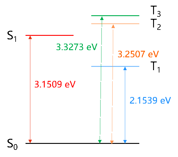
- target:
3.2-1
The strength of the transition between two states can be measured by the oscillator strength, which is a dimensionless quantity. The expression for the oscillator intensity of the |i> → |j> transition in atomic units is .. math:
f_{ij} = 2/3(E_{j}-E_{i})|<i|-r|j>|^2
where
where :math:’rm E_{j}’ and :math:’rm E_{i}’ are the energies of the two states, respectively. The greater the oscillator strength between the ground state and an excited state, the easier it is to absorb electromagnetic waves of the corresponding frequency and transition to that excited state, and the stronger the corresponding absorption peak in the absorption spectrum. In general, an oscillator strength of less than 0.001 can be considered a transition prohibition.
The low excited state excitation energy, oscillator strength, and transition dipole moment are shown in the table.
- Excited state Excitation energy/eV oscillator strength Transition dipole moment/Debye
S1
3.1509
0.6012
19.7948
T1
2.1539
0.0000
0.0000
T2
3.2507
0.0000
0.0000
The absorption spectra plotted are as follows.
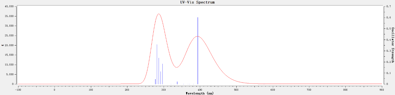
Convert the chk file to the fchk file. Render NTO tracks with Multiwfn VMD.
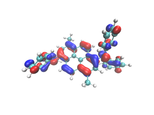
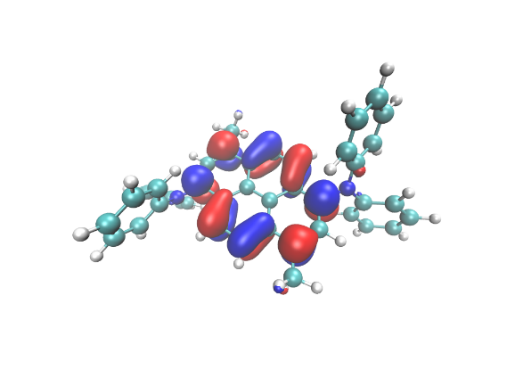
\(\rm S_{0}\) → \(\rm S_{1}\) The NTO contribution to the transition with the largest contribution is 96.40%.
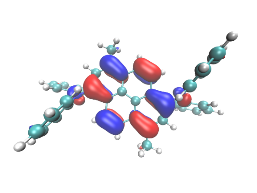
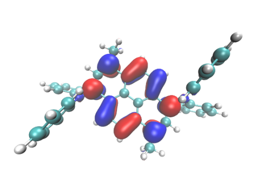
\(\rm S_{0}\) → \(\rm T_{1}\) The NTO contribution to the transition with the largest contribution was 95.52%.
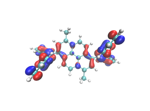
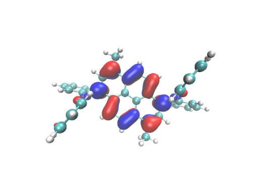
\(\rm S_{0}\) → :math:`rm T_{2}`The NTO contribution to the transition was 86.41%.
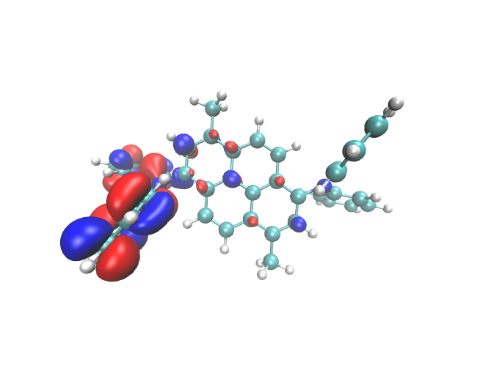
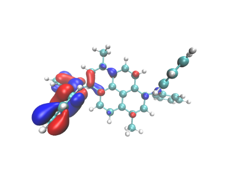
\(\rm S_{0}\) → \(\rm T_{3}\) transition contributes most to NTO pairs with a contribution value of 62.93%.
As can be seen from the diagram, the :math:’rm T_{1}’ and :math:’rm T_{3}’ states are typical local excitation (LE), while the :math:’rm S_{1}’ and :math:’rm T_{2}’ states have both charge transfer and local excitation components, which belong to the HLCT state.
Excited state :math:’rm S_{1}’ optimization
Fluorescence is a cold light phenomenon that generally refers to the radiation process that occurs between spin singlet states. According to the Kasha rule, it is the emission from the lowest excited state to the ground state, which is generally from the :math:’rm S_{1}’ state to the :math:’rm S_{0}’ state. In order to simulate the fluorescence process, it is also necessary to optimize the structure and frequency of the excited state :math:’rm S_{1}’, and obtain the ‘’log’’ file and ‘’fchk’’ file to prepare for the subsequent MOMAP calculation. The functional and base groups are M062x and Def2SVP, respectively, and the ‘’gjf’’ file is as follows:
%nprocshared=32
%mem=6GB
%chk=s1opt.chk
#P opt freq M062x/Def2SVP TD(nstates=3,root=1)

Title Card Required

0 1
 C                  1.565649   -4.134284   -0.176953
 C                  1.643599   -2.628388   -0.152751
 C                  2.886000   -2.003080   -0.112539
 C                  3.020859   -0.613479   -0.088550
 N                  4.325420   -0.044576   -0.036499
 C                  5.278240   -0.466495   -0.995386
 C                  4.884618   -0.626003   -2.332720
 C                  5.799622   -1.064339   -3.285338
 C                  7.121820   -1.335486   -2.928150
 C                  7.515238   -1.172730   -1.598991
 C                  6.603320   -0.752040   -0.633991
 C                  4.698175    0.744156    1.076980
 C                  4.091832    0.542012    2.325047
 C                  4.427797    1.352319    3.406784
 C                  5.379893    2.362883    3.271786
 C                  5.988191    2.561344    2.030562
 C                  5.647767    1.769732    0.937881
 C                  1.876752    0.211899   -0.120738
 C                  0.588755   -0.407573   -0.126231
 C                  0.473733   -1.832327   -0.148612
 C                 -0.837555   -2.410247   -0.178205
 C                 -1.959943   -1.640762   -0.161854
 C                 -1.876694   -0.212016   -0.120592
 C                 -0.588696    0.407452   -0.126517
 C                 -0.473668    1.832190   -0.149905
 C                  0.837623    2.410088   -0.179888
 C                  1.960009    1.640614   -0.162984
 C                 -1.643530    2.628249   -0.154622
 C                 -2.885933    2.002973   -0.113981
 C                 -3.020804    0.613392   -0.088992
 N                 -4.325380    0.044559   -0.036541
 C                 -4.698230   -0.743314    1.077511
 C                 -4.091928   -0.540291    2.325457
 C                 -4.428022   -1.349755    3.407783
 C                 -5.380213   -2.360326    3.273499
 C                 -5.988485   -2.559645    2.032401
 C                 -5.647934   -1.768883    0.939143
 C                 -5.278162    0.465750   -0.995788
 C                 -4.884527    0.624147   -2.333249
 C                 -5.799513    1.061738   -3.286228
 C                 -7.121702    1.333222   -2.929264
 C                 -7.515137    1.171550   -1.599978
 C                 -6.603236    0.751616   -0.634632
 C                 -1.565577    4.134127   -0.179894
 H                  2.565826   -4.573123   -0.163055
 H                  1.054624   -4.497512   -1.075888
 H                  1.015461   -4.526102    0.685940
 H                  3.789152   -2.604760   -0.095814
 H                  3.860188   -0.404796   -2.611283
 H                  5.478783   -1.182339   -4.316028
 H                  7.834889   -1.669709   -3.674725
 H                  8.537506   -1.389762   -1.303667
 H                  6.910123   -0.642734    0.399820
 H                  3.355698   -0.245579    2.436971
 H                  3.946094    1.182749    4.365139
 H                  5.642450    2.988231    4.118776
 H                  6.724707    3.349483    1.905053
 H                  6.110094    1.939850   -0.027830
 H                 -0.934317   -3.489037   -0.217496
 H                 -2.937842   -2.104213   -0.185630
 H                  0.934386    3.488850   -0.219935
 H                  2.937915    2.104041   -0.187063
 H                 -3.789080    2.604673   -0.097685
 H                 -3.355727    0.247315    2.436831
 H                 -3.946346   -1.179515    4.366033
 H                 -5.642871   -2.985014    4.120945
 H                 -6.725084   -3.347795    1.907449
 H                 -6.110250   -1.939666   -0.026456
 H                 -3.860104    0.402673   -2.611627
 H                 -5.478667    1.178888   -4.317013
 H                 -7.834757    1.666861   -3.676114
 H                 -8.537402    1.388848   -1.304838
 H                 -6.910046    0.643140    0.399265
 H                 -1.015334    4.526556    0.682686
 H                 -2.565752    4.572979   -0.166245
 H                 -1.054607    4.496714   -1.079120
After the job is completed, find the last excited state in the log file 1 is :math:’rm S_{1}’ excitation energy, and Total Energy is the electronic state energy.
Excited State   1:      Singlet-A      2.7938 eV  443.79 nm  f=0.8006  <S**2>=0.000
149 ->150         0.69410
This state for optimization and/or second-order correction.
Total Energy, E(TD-HF/TD-DFT) =  -1727.22867894
Copying the excited state density for this state as the 1-particle RhoCI density.
Excited state \(\rm T_{2}\), \(\rm T_{3}\) optimization ——————————————-——————————————————————————————————————————————————————————————
Since MOMAP will be used to calculate the inter-system crossing rate of :math:’rm T_{2}’ → :math:’rm S_{1}’ states and :math:’rm T_{3}’ → :math:’rm S_{1}’ states in the early stage, it is also necessary to optimize the structure and frequency calculation of excited states :math:’rm T_{2}’ and :math:’rm T_{3}’ to obtain ‘log’’ files and ‘’ FCHK’’ file. The functional and base groups are M062x and Def2SVP, respectively, and the T2.gjf file is as follows:
%nprocshared=32
%mem=6GB
%chk=t2.chk
#P opt freq M062x/Def2SVP TD(triplets,nstates=6,root=2)

Title Card Required

0 1
 C                  1.565649   -4.134284   -0.176953
 C                  1.643599   -2.628388   -0.152751
 C                  2.886000   -2.003080   -0.112539
 C                  3.020859   -0.613479   -0.088550
 N                  4.325420   -0.044576   -0.036499
 C                  5.278240   -0.466495   -0.995386
 C                  4.884618   -0.626003   -2.332720
 C                  5.799622   -1.064339   -3.285338
 C                  7.121820   -1.335486   -2.928150
 C                  7.515238   -1.172730   -1.598991
 C                  6.603320   -0.752040   -0.633991
 C                  4.698175    0.744156    1.076980
 C                  4.091832    0.542012    2.325047
 C                  4.427797    1.352319    3.406784
 C                  5.379893    2.362883    3.271786
 C                  5.988191    2.561344    2.030562
 C                  5.647767    1.769732    0.937881
 C                  1.876752    0.211899   -0.120738
 C                  0.588755   -0.407573   -0.126231
 C                  0.473733   -1.832327   -0.148612
 C                 -0.837555   -2.410247   -0.178205
 C                 -1.959943   -1.640762   -0.161854
 C                 -1.876694   -0.212016   -0.120592
 C                 -0.588696    0.407452   -0.126517
 C                 -0.473668    1.832190   -0.149905
 C                  0.837623    2.410088   -0.179888
 C                  1.960009    1.640614   -0.162984
 C                 -1.643530    2.628249   -0.154622
 C                 -2.885933    2.002973   -0.113981
 C                 -3.020804    0.613392   -0.088992
 N                 -4.325380    0.044559   -0.036541
 C                 -4.698230   -0.743314    1.077511
 C                 -4.091928   -0.540291    2.325457
 C                 -4.428022   -1.349755    3.407783
 C                 -5.380213   -2.360326    3.273499
 C                 -5.988485   -2.559645    2.032401
 C                 -5.647934   -1.768883    0.939143
 C                 -5.278162    0.465750   -0.995788
 C                 -4.884527    0.624147   -2.333249
 C                 -5.799513    1.061738   -3.286228
 C                 -7.121702    1.333222   -2.929264
 C                 -7.515137    1.171550   -1.599978
 C                 -6.603236    0.751616   -0.634632
 C                 -1.565577    4.134127   -0.179894
 H                  2.565826   -4.573123   -0.163055
 H                  1.054624   -4.497512   -1.075888
 H                  1.015461   -4.526102    0.685940
 H                  3.789152   -2.604760   -0.095814
 H                  3.860188   -0.404796   -2.611283
 H                  5.478783   -1.182339   -4.316028
 H                  7.834889   -1.669709   -3.674725
 H                  8.537506   -1.389762   -1.303667
 H                  6.910123   -0.642734    0.399820
 H                  3.355698   -0.245579    2.436971
 H                  3.946094    1.182749    4.365139
 H                  5.642450    2.988231    4.118776
 H                  6.724707    3.349483    1.905053
 H                  6.110094    1.939850   -0.027830
 H                 -0.934317   -3.489037   -0.217496
 H                 -2.937842   -2.104213   -0.185630
 H                  0.934386    3.488850   -0.219935
 H                  2.937915    2.104041   -0.187063
 H                 -3.789080    2.604673   -0.097685
 H                 -3.355727    0.247315    2.436831
 H                 -3.946346   -1.179515    4.366033
 H                 -5.642871   -2.985014    4.120945
 H                 -6.725084   -3.347795    1.907449
 H                 -6.110250   -1.939666   -0.026456
 H                 -3.860104    0.402673   -2.611627
 H                 -5.478667    1.178888   -4.317013
 H                 -7.834757    1.666861   -3.676114
 H                 -8.537402    1.388848   -1.304838
 H                 -6.910046    0.643140    0.399265
 H                 -1.015334    4.526556    0.682686
 H                 -2.565752    4.572979   -0.166245
 H                 -1.054607    4.496714   -1.079120
After the job is completed, find the last excited state in the log file 2 is :math:’rm T_{2}’ excited energy, and Total Energy is the electronic state energy.
Excited State   2:      Triplet-A      3.0388 eV  408.01 nm  f=0.0000  <S**2>=2.000
138 ->150        -0.14038
148 ->150         0.61959
149 ->155         0.16846
149 ->157        -0.14448
This state for optimization and/or second-order correction.
Total Energy, E(TD-HF/TD-DFT) =  -1727.22151297
Copying the excited state density for this state as the 1-particle RhoCI density.
Similarly, optimizing :math:’rm T_{3}’ yields the energy of the :math:’rm T_{3}’ state. The results show that the energy of the electronic state of :math:’rm T_{3}’ is less than that of the :math:’rm T_{2}’ state, which means that the energy of the :math:’rm T_{2}’ and :math:’rm T_{3}’ states may cross in the process of optimization away from the Frank-Condon zone, so that the energy of the final optimized :math:’rm T_{3}’ minimum point is less than that of :math:’rm T_{2}’. .. code-block:: bdf
Excited State 3: Triplet-A 2.9283 eV 423.40 nm f=0.0000 <S**2>=2.000 149 ->151 0.67322 149 ->155 0.11403 This state for optimization and/or second-order correction. Total Energy, E(TD-HF/TD-DFT) = -1727.22240086 Copying the excited state density for this state as the 1-particle RhoCI density.
Spin orbit coupling
Spin-orbit coupling (SOC) reflects the interaction between the spin of an electron and the rotation of an electron around the nucleus. When calculating the transitions between the singlet and triplet states, if the spin-orbit coupling is not considered (i.e., the coupling is strictly 0), then their transitions are forbidden. However, when the rotary-orbit coupling is introduced into the Hamiltonian, the coupling between the two states is not strictly 0, and the transition between the singlet and triplet states is possible. We tend to be concerned with the spin-orbit coupling between the :math:’rm S_{i}’ state and the :math:’rm T_{j}’ state in a particular structure. where :math:’rm <S_{i}|SOC|T_{j}>’ denotes the spin-orbit coupling matrix element, which is measured by its modulus to measure the size of the spin-orbit coupling between the :math:’rm S_{i}’ and :math:’rm T_{j}’ electronic states. This physical quantity can also be used to calculate the intersystem crossing (ISC) rate and the reverse intersystem crossing (RISC) rate.
In this example, BDF is used to calculate the spin-orbit coupling matrix element between the :math:’rm S_{1}’ - :math:’rm T_{2}’ and :math:’rm S_{1}-T_{3}’ states, using the M062x functional, Def2SVP basis set, and the ‘’inp’’ file is as follows:
$compass
Title
  C42H32N2
Geometry
 C                  1.586003   -4.127364   -0.277679
 C                  1.687147   -2.632259   -0.222611
 C                  2.912299   -2.005731   -0.177241
 C                  3.045692   -0.604559   -0.100709
 N                  4.333135   -0.047256   -0.013973
 C                  5.334680   -0.519389   -0.889609
 C                  5.015755   -0.759732   -2.235838
 C                  5.984347   -1.247032   -3.105784
 C                  7.281444   -1.498204   -2.653995
 C                  7.598599   -1.262567   -1.315545
 C                  6.635646   -0.783602   -0.432749
 C                  4.653716    0.850763    1.024080
 C                  3.972142    0.778096    2.248981
 C                  4.252686    1.694201    3.257436
 C                  5.214213    2.687133    3.070218
 C                  5.894013    2.759318    1.852004
 C                  5.615474    1.857669    0.831601
 C                  1.878302    0.232663   -0.125495
 C                  0.592246   -0.400870   -0.142073
 C                  0.488519   -1.828638   -0.190107
 C                 -0.793696   -2.412608   -0.223962
 C                 -1.944019   -1.641486   -0.186177
 C                 -1.878300   -0.232665   -0.125495
 C                 -0.592244    0.400868   -0.142073
 C                 -0.488517    1.828637   -0.190108
 C                  0.793698    2.412606   -0.223963
 C                  1.944022    1.641485   -0.186177
 C                 -1.687145    2.632258   -0.222613
 C                 -2.912297    2.005730   -0.177243
 C                 -3.045690    0.604558   -0.100710
 N                 -4.333133    0.047256   -0.013974
 C                 -4.653717   -0.850761    1.024079
 C                 -3.972142   -0.778097    2.248980
 C                 -4.252689   -1.694201    3.257435
 C                 -5.214220   -2.687128    3.070218
 C                 -5.894022   -2.759311    1.852005
 C                 -5.615479   -1.857663    0.831601
 C                 -5.334678    0.519389   -0.889611
 C                 -5.015753    0.759734   -2.235839
 C                 -5.984345    1.247034   -3.105785
 C                 -7.281443    1.498203   -2.653996
 C                 -7.598599    1.262562   -1.315546
 C                 -6.635645    0.783598   -0.432750
 C                 -1.586001    4.127363   -0.277682
 H                  2.581935   -4.588013   -0.284388
 H                  1.048934   -4.459802   -1.181513
 H                  1.027774   -4.525258    0.585788
 H                  3.824462   -2.607245   -0.175768
 H                  4.002023   -0.553508   -2.582465
 H                  5.725422   -1.423160   -4.150923
 H                  8.039250   -1.878188   -3.339953
 H                  8.605471   -1.467565   -0.948393
 H                  6.879710   -0.616710    0.617096
 H                  3.223855   -0.001794    2.394755
 H                  3.715870    1.625084    4.204829
 H                  5.431113    3.401551    3.864968
 H                  6.641732    3.536971    1.688418
 H                  6.130708    1.931595   -0.127046
 H                 -0.888701   -3.496890   -0.277700
 H                 -2.914627   -2.134719   -0.218301
 H                  0.888703    3.496889   -0.277701
 H                  2.914629    2.134717   -0.218301
 H                 -3.824459    2.607244   -0.175771
 H                 -3.223853    0.001791    2.394754
 H                 -3.715872   -1.625085    4.204828
 H                 -5.431123   -3.401546    3.864969
 H                 -6.641744   -3.536960    1.688420
 H                 -6.130714   -1.931587   -0.127046
 H                 -4.002021    0.553512   -2.582466
 H                 -5.725421    1.423163   -4.150924
 H                 -8.039249    1.878187   -3.339954
 H                 -8.605471    1.467558   -0.948395
 H                 -6.879709    0.616703    0.617094
 H                 -1.027772    4.525257    0.585785
 H                 -2.581933    4.588012   -0.284392
 H                 -1.048931    4.459800   -1.181516
End Geometry
Basis
  Def2-SVP
Skeleton
Group
  C(1)
$end

$xuanyuan
Heff
  21
Hsoc
  2
Direct
RS
  0.33
$end

$scf
RKS
Charge
  0
SpinMulti
  1
DFT
  M062X
MPEC+COSX
Molden
$end

$tddft
Imethod
  1
Isf
  0
Idiag
  1
Iroot
  3
MPEC+COSX
Istore
  1
$end

$tddft
Imethod
  1
Isf
  1
Idiag
  1
Iroot
  3
MPEC+COSX
Istore
  2
$end

$tddft
Isoc
  2
Nfiles
  2
Ifgs
  1
Imatsoc
  2
1 1 1 2 1 2
1 1 1 2 1 3
$end
After the job is completed, the following keywords are found in the ‘’out’ output file, which is the rotary-orbit coupling matrix element result
[tddft_soc_matsoc]

 Print selected matrix elements of [Hsoc]

 SocPairNo. =    1   SOCmat = <  1  1  1 |Hso|  2  1  2 >     Dim =    1    3
   mi/mj          ReHso(au)       cm^-1               ImHso(au)       cm^-1
  0.0 -1.0     -0.0000031365     -0.6883766845      0.0000019744      0.4333410617
  0.0  0.0      0.0000000000      0.0000000000     -0.0000000001     -0.0000289692
  0.0  1.0     -0.0000031365     -0.6883766845     -0.0000019744     -0.4333410617

 SocPairNo. =    2   SOCmat = <  1  1  1 |Hso|  2  1  3 >     Dim =    1    3
   mi/mj          ReHso(au)       cm^-1               ImHso(au)       cm^-1
  0.0 -1.0     -0.0000000002     -0.0000481328      0.0000000002      0.0000411125
  0.0  0.0      0.0000000000      0.0000000000     -0.0000069588     -1.5272872617
  0.0  1.0     -0.0000000002     -0.0000481328     -0.0000000002     -0.0000411125
Here :math:’rm SOCmat=<1 1 1 |H_{SO}| 2 1 2>’ represents the matrix element :math:’rm <S_{1}| H_{SO} |T_{2}>’ , ReHso and ImHso represent the real and imaginary parts, respectively, in au or :math:’rm cm^{-1}’. After summing the modulus squares of the SOC matrix elements of the three mj components, and then opening the square to obtain the coupling matrix element of the :math:’rm S_{1}’ state and the :math:’rm T_{2}’ state of the subsequent MOMAP, that is, 1.15035 :math:’rm cm^{-1}’; :math:’rm S_{1}’ state and :math:’rm T_{3}’ state spin-orbit coupling matrix element 1.52729 :math:’rm cm^{-1}’.
Reforming energy
The reforming energy refers to the change in the energy of the system due to the relaxation of the geometric structure when the molecule gains and loses electrons. It is not only a key physical quantity that affects the electron transfer rate (based on the Marcus theory), but also an important factor affecting the spectral spectrum and radiation rate. Specifically, the energy difference between the initial and final states of a molecule is the reforming energy of the ground state and the excited state, respectively: math:’lambda_{S0}=E_{3}-E_{1}’ , :math:’lambda_{S1}=E_{2}-E_{4}’.
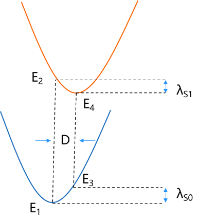
Reforming energy can also be defined as:
where :math:’rm S_k’ and :math:’rm ω_k’ are the Huang−Rhys factor and frequency of the k-th mode, respectively, and D is the mode shift.
Huang Kun factor
The input files require the structural optimization and frequency calculation log files and fchk files of :math:’rm S_0’ and :math:’rm S_1’, as well as the momap.inp’ file and the momap.inp file, as follows:
do_evc            = 1

&evc
  ffreq(1)      = "s0.log"
  ffreq(2)      = "s1.log"
  set_cart = t
/
After the job is completed, the evc.cart.dat’ file is generated, and the following keywords are found to be the restructure energy of :math:’rm S_0’ and :math:’rm S_1’. As shown in the figure below, :math:’lambda_{S0} = 1610.605 cm^{−1}’ , :math:’lambda_{S1} = 1864.085 cm^{−1}’, that is, the ground state and excited state reforming energies are not much different, indicating that the two state configurations are not much different and belong to the same Franck-Condon region.
Total reorganization energy (cm-1): 1610.605075 1864.085048
Opening the evc.cart.dat file in Device Studio gives the :math:’rm S_0 state and the :math:rm S_1 state rewhole energy and the contribution of the Huang Kun factor in each vibration mode.
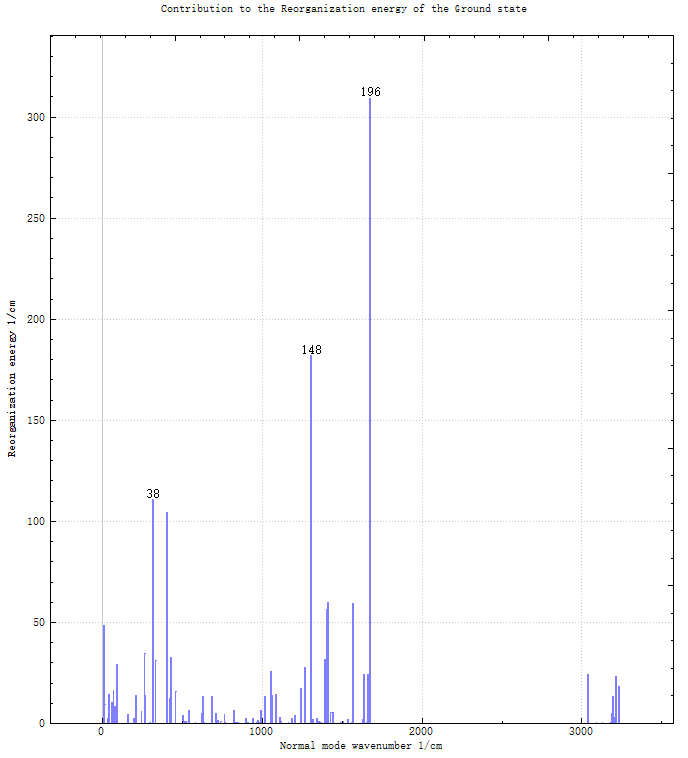
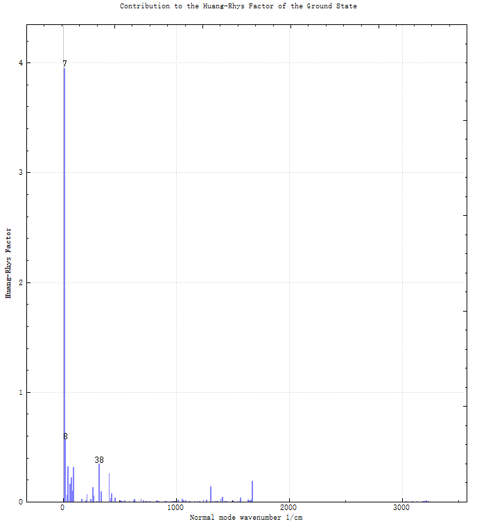
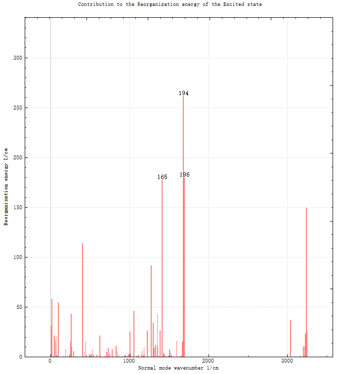
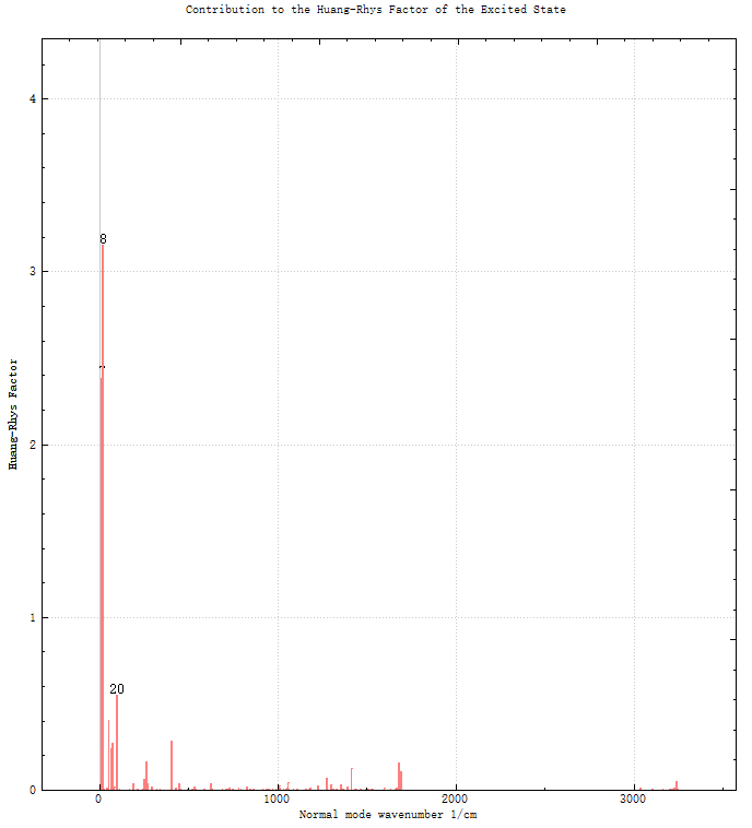
The vibration modes are analyzed, and it is found that the main contribution of the recombination energy of the :math:’rm S_{0}’ state comes from the high-frequency C-C telescopic vibration of 1676.69 :math:’rm cm^{-1}’ and the high-frequency bending vibration of 1308.32 :math:’rm cm^{-1}’, and the main contribution of the recombination energy of the :math:’rm S_1’ state comes from 1683.31 :math:’rm cm^{-1}’ and 1695.91 : Math:’rm cm^{-1}’ and 1414.86:math:’rm cm^{-1}’. The maximum mode of the Huangkun factor in the :math:’rm S_{0}’ state is 12.24 :math:’rm cm^{-1}’, and the maximum mode of the Huangkun factor in the S1 state is 18.30 :math:’rm cm^{-1}’.
In the photophysical process of molecules, the Duschinsky rotation effect caused by the overlap between the regular modes of the transition initial state and the final state will also have an important impact on the spectrum and rate, the 3N-6 regular coordinates obtained at the S0 and S1 minima are different, and they are linear transformation relations with each other, which can be expressed as Q’’=J*Q’ ΔQ, where Q’ and Q’’ represent the regular modes at the two electronic minima respectively, J is called the Duschinsky matrix. Open the evc.cart.abs file in Device Studio to get a 2D plot of the Duschinsky rotation matrix between the S0 and S1 states.

Fluorescence spectroscopy
The calculation of the fluorescence radiation rate with MOMAP requires the results of the previous step “evc.cart.dat’” and the new input files “momap.inp” and “momap.inp” which are as follows:
do_spec_tvcf_ft   = 1
do_spec_tvcf_spec = 1

&spec_tvcf
  DUSHIN        = .t.
  Temp          = 300 K
  tmax          = 1000 fs
  dt            = 1   fs
  Ead           = 0.09626 au
  EDMA          = 8.18309 debye
  EDME          = 9.64296 debye
  FreqScale     = 1.0
  DSFile        = "evc.cart.dat"
  Emax          = 0.3 au
  dE            = 0.00001 au
  logFile       = "spec.tvcf.log"
  FtFile        = "spec.tvcf.ft.dat"
  FoFile        = "spec.tvcf.fo.dat"
  FoSFile       = "spec.tvcf.spec.dat"
/
For the adiabatic excitation energy Ead, since Gaussian uses different calculation levels to calculate :math:’rm S_0 and :math:’rm S_1’, we use the structure of :math:’rm S_1’ to do a single point calculation at the calculation level of :math:’rm S_0’ for correction: with this energy - :math:’rm S_0’ energy :math:’rm S_1’ The excitation energy yields the adiabatic excitation energy, i.e., Ead=0.09626 au. For the absorption transition dipole moment EDMA, read the first ground state to the excited state transition electric dipole moment Dip.S. from the S1.log file, and convert the root number and units to obtain 8.18309 debye. For the emission transition dipole moment EDME, 9.64296 debye is obtained by reading the last ground state to the excited state transition electric dipole moment Dip.S. from the S1.log file, and the root number is converted into units. (The results of Ead, EDMA and EDME were obtained under the condition of adding benzene solvent (scrf(solvent=benzene, SMD)) to simulate the thin film environment).
After the job is completed, the radiation rate can be read at the end of the spec.tvcf.log file, in this case :math:’rm S_1’ → :math:’rm S_0’ The radiation rate is :math:’rm 1.77 times 10^8 s^{-1}’ and the fluorescence lifetime is 5.64 ns.
  I^-1 =     3.05463233E+00 Hartree =    6.70414303E+05 cm-1 =   8.31208105E+01 eV

radiative rate     (0):     4.28614462E-09    1.77195105E+08 /s,       5.64 ns
Open the spec.tvcf.spec.dat file in Device Studio to obtain the absorption and emission spectra, as shown below, with the absorption at 388 nm and the emission at 497 nm.
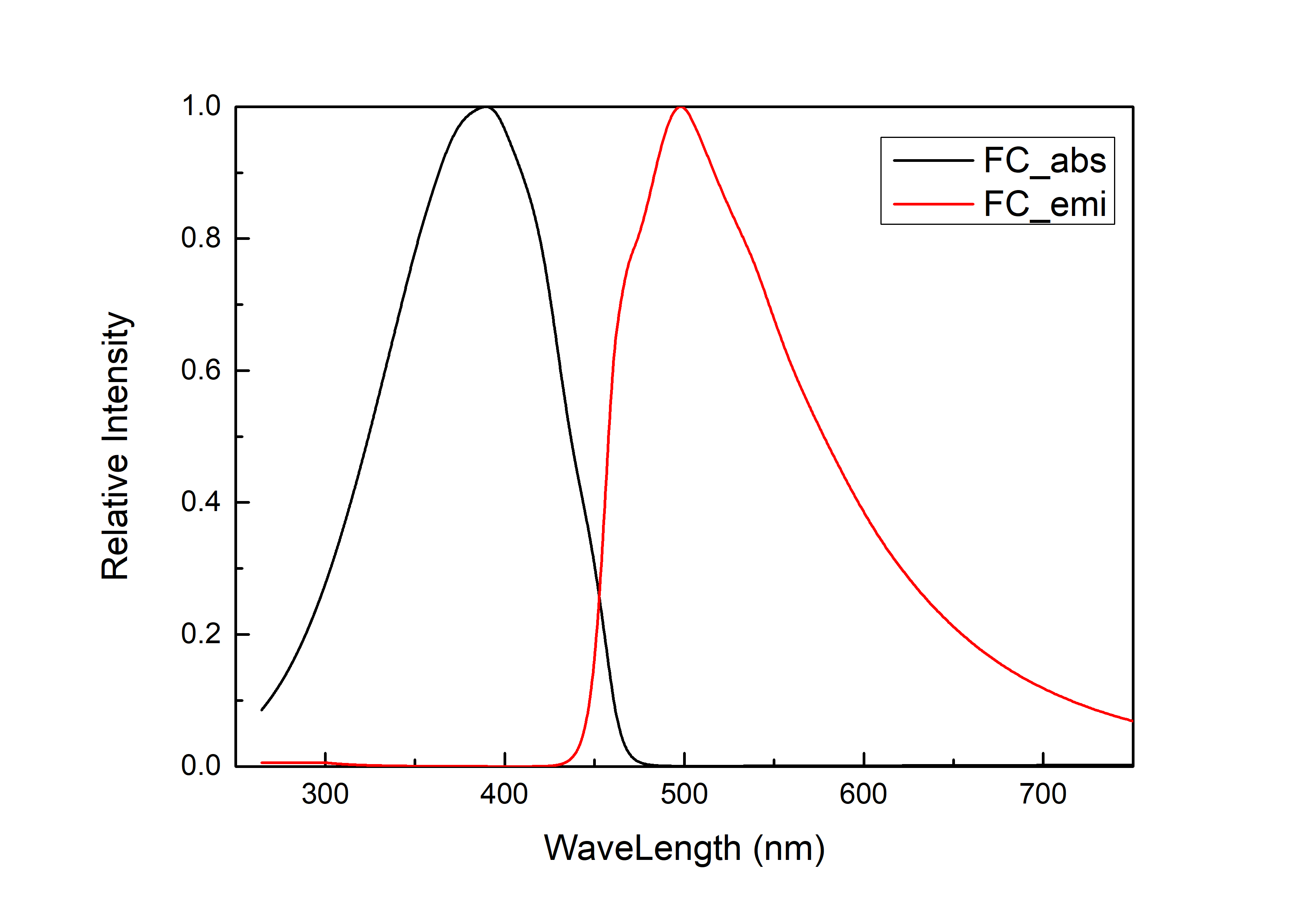
The rate of inter-system channeling
Intersystem channeling is an important radiation-free process in photochemistry. It refers to the fact that after the molecule is excited, due to the intersection between the potential energy surfaces of states with different spin multiplicities, the spin multiplicity changes in a non-radiative way when the system undergoes such a structure. In general organic systems, RISC refers to the transition from a single to a triplet state, and reverse RISC refers to the transition from a triplet to a singlet state. The inter-system crossing rate, e.g. :math:’rm S_0 → t_2’, is also related to their energy level difference :math:’Delta E_{ST}’. Here :math:’Delta E_{ST}’ can be obtained by subtracting the excited state energy of :math:’rm S_{1}’ from the excited state energy of :math:’rm T_{2}’. Calculate :math:’rm S_1 - T_2’ state :math:’Delta E_{ST}’ =0.05518 au, :math:’rm S_1 - T_3’ state :math:’Delta E_{ST}’ =0.05528 au.
In order to calculate the inter-system channeling rate in the MOMAP program, you first need to calculate the electronic vibration coupling of :math:’rm S_1’ and :math:’rm T_2’, the file needs the log frequency calculation files of :math:’rm S_1’ and :math:’rm T_2’ and the fchk file, as well as the momap.inp input file, and the momap.inp file as follows:
do_evc            = 1

&evc
  ffreq(1)      = "s1.log"
  ffreq(2)      = "t2.log"
  set_cart = t
/
After the job is completed, the generated evc.cart.dat file is placed in the same directory as the new momap.inp file to calculate the non-radiometric rate. The input file ‘’momap.inp’’ is as follows:
do_isc_tvcf_ft   = 1
do_isc_tvcf_spec = 1

&isc_tvcf
   DUSHIN    = .t.
   Temp      = 298 K
   tmax      = 1500 fs
   dt        = 1 fs
   Ead       = 0.05518 au
   Hso       = 1.15035 cm-1
   DSFile    = "evc.cart.dat"
   Emax      = 0.3 au
   logFile   = "isc.tvcf.log"
   FtFile    = "isc.tvcf.ft.dat"
   FoFile    = "isc.tvcf.fo.dat"
/
Ead is \(\Delta E_{ST}\) , \(rm H_{SO}\) is the \(rm S_1\) state and \(rm T_2\) state spin-orbit coupling matrix element, and the calculated isc.tvcf.log file ends with the intersystem channeling rate and the anti-system channeling rate, in this case \(rm k_{ISC} = 4.53 times 10^4 s^{-1}\) , \(k_{RISC} = 1.48 times 10^2 s^{-1}\), where Ead is the energy difference between the singlet and triplet states, H_SO is the spin-orbit coupling matrix element between the S_1 and T_2 states.
#         Intersystem crossing Ead is      0.0551800 au, rate is    4.53103856E+04 s-1, lifetime is    2.20699954E-05 s
# Reverse Intersystem crossing Ead is     -0.0551800 au, rate is    1.47691362E+02 s-1, lifetime is    6.77087667E-03 s
Similarly, the inter-system crossing rate between the :math:’rm S_1’ state and the :math:’T_3’ state is :math:’rm k_{ISC} = 8.75 times 10^7 s^{-1}’ and the anti-system crossing rate :math:’rm k_{ISC} = 1.32 times 10^7 s^{-1}’.
#         Intersystem crossing Ead is      0.0552800 au, rate is    8.75255907E+07 s-1, lifetime is    1.14252300E-08 s
# Reverse Intersystem crossing Ead is     -0.0552800 au, rate is    1.31729899E+07 s-1, lifetime is    7.59129104E-08 s
Through calculation, we find that the anti-system crossing rate between the :math:’rm T_2’ state and the :math:’rm S_1’ state is very small, which does not meet the requirements of HLCT molecules. The anti-system crossing rate from the :math:’rm T_3’ state to the :math:’rm S_1’ state is large, indicating that the triplet exciton may undergo anti-system crossing in the :math:’rm T_3’ state and transform into the :math:’rm S_1’ state.
conclusion
In this paper, based on the DFT and TDDFT theories, the excited photophysical processes of 2TPA-Py molecules are calculated. The results show that the :math:’rm S_1’ state of 2TPA-Py molecule has the characteristics of HLCT, and its maximum emission wavelength is sky blue at 497 nm. The inter-anti-transparency rate of :math:’rm T_3 → S_1’ of this molecule is as high as :math:’4.39 times 106 s^{-1}’, which basically satisfies the requirement of utilizing triplet excitons through anti-inter-transgression. It can be seen that the molecular design strategy of donor-π-donor is expected to be an effective means to construct high-stability blue light HLCT molecules.
Theoretical Investigation of Phosphorescence Emission Mechanism in Ir(ppy)₃
Since phosphorescent materials were applied to OLEDs, research on organic light-emitting devices based on phosphorescence mechanisms has developed rapidly, including representative red, green, and blue monochromatic phosphorescent devices and full-phosphorescent white OLEDs. Due to spin-forbidden transitions, phosphorescence quantum yields are generally much lower than fluorescence. Therefore, methods such as the heavy atom effect are typically employed to enhance phosphorescence quantum yield. When heavy atoms are introduced, spin-orbit coupling strengthens, making the forbidden triplet-to-singlet transitions allowed. This significantly reduces the time molecules remain in the triplet state and greatly improves the internal quantum efficiency of devices. Commonly used heavy metal atoms include Ir, Pt, Re, Os, Cu, etc.
Phosphorescent materials should generally possess good photothermal stability, large molecular absorption cross-sections, high intersystem crossing ability, high phosphorescence quantum yields at room temperature, and short triplet lifetimes. Since green phosphorescent materials are easiest to obtain among organic materials, research began with phosphorescent green OLEDs. Among them, Ir(ppy)₃ is the most representative material and has been widely used in phosphorescent devices. The phosphorescence emission rate is an important parameter in luminescence mechanism research. This article will use Ir(ppy)₃ as an example to calculate its phosphorescence emission rate using BDF and MOMAP software. First, structural optimization, frequency calculation, and spin-orbit coupling calculation need to be performed using BDF quantum software. Then, based on BDF’s structural optimization and frequency calculation result files, and spin-orbit coupling calculation result files, MOMAP software will be used to calculate the phosphorescence radiative rate.
Ground State Optimization
First, use BDF quantum software to perform structural optimization and frequency calculation for Ir(ppy)₃’s ground state S₀ and first triplet excited state T₁.
Prepare the xyz file of Ir(ppy)₃’s molecular structure:
61

Ir   -2.606160230000     -0.262817540000      0.032585640000
C    -3.837298770000      2.407777490000      0.243683290000
C    -1.553000180000      2.622608110000      0.521271830000
C    -3.991643180000      3.786525490000      0.422094600000
C    -4.929719550000      1.476909230000     -0.003856060000
C    -1.634158680000      3.988444110000      0.709067180000
H    -0.591261780000      2.126459120000      0.554253960000
C    -2.889293280000      4.581787990000      0.656041260000
H    -4.972006580000      4.231616950000      0.376099570000
C    -6.263398690000      1.888616610000     -0.076321100000
H    -0.744068550000      4.570116630000      0.889344200000
H    -2.999939670000      5.647195600000      0.795286530000
C    -5.623129880000     -0.778047400000     -0.424041550000
C    -7.264449980000      0.973962040000     -0.319493370000
H    -6.527094820000      2.928025340000      0.057085040000
C    -6.940359500000     -0.364034500000     -0.495248330000
H    -5.397358100000     -1.824987250000     -0.570011260000
H    -8.293855190000      1.298147200000     -0.375111620000
H    -7.723296650000     -1.084118350000     -0.689505650000
C    -2.780095460000     -2.271307610000     -0.073978550000
C    -2.962145630000     -2.905938610000      1.179649240000
C    -2.704720750000     -3.101798200000     -1.194651040000
C    -3.053849400000     -4.297470620000      1.273150410000
C    -3.052375550000     -2.037406190000      2.345262930000
C    -2.797310890000     -4.477732940000     -1.095358170000
H    -2.574810200000     -2.657655530000     -2.171485550000
C    -2.970830350000     -5.080470100000      0.142706420000
H    -3.190782260000     -4.777448690000      2.231582660000
C    -3.251325250000     -2.483356810000      3.656088400000
H    -2.735191030000     -5.089028800000     -1.985144810000
H    -3.042943740000     -6.155896270000      0.221114210000
C    -2.995026490000      0.148733040000      3.092507280000
C    -3.319187740000     -1.576319800000      4.692855730000
H    -3.353725050000     -3.536644150000      3.859562860000
C    -3.186631940000     -0.222801710000      4.408749290000
H    -2.888815760000      1.194668600000      2.833837140000
H    -3.472767910000     -1.912494740000      5.707724440000
H    -3.232610730000      0.522480480000      5.186904590000
N    -2.927015180000     -0.717593640000      2.090156960000
C     0.125501920000     -0.309636820000     -1.075330180000
C     0.242318970000     -0.710559210000      1.197687130000
C     1.518232510000     -0.401785790000     -1.166132500000
C    -0.762473880000     -0.044853840000     -2.198985150000
C     1.619464440000     -0.811598610000      1.179643800000
H    -0.298309850000     -0.828666640000      2.128258480000
C     2.270161400000     -0.653514600000     -0.037593100000
H     2.007628100000     -0.277927520000     -2.118201950000
C    -2.150460220000     -0.005742870000     -1.917121780000
C    -0.287950380000      0.157363030000     -3.497950870000
H     2.165728000000     -1.009392350000      2.088259610000
H     3.346017750000     -0.726918300000     -0.099292420000
C    -3.004998770000      0.237880450000     -2.994864780000
C    -1.165335710000      0.397865570000     -4.532504760000
H     0.771521710000      0.127613130000     -3.708268180000
C    -2.529020200000      0.436535570000     -4.277665910000
H    -4.071982740000      0.267717660000     -2.824596670000
H    -0.792761550000      0.552584980000     -5.535050450000
H    -3.220629300000      0.622039860000     -5.087916480000
N    -0.487689310000     -0.467248190000      0.117089220000
N    -2.608631830000      1.850704260000      0.298598520000
C    -4.578169480000      0.115167240000     -0.176155400000
Open Device Studio, click File → New Project, name it phosphorescence.hpf, drag Ir(ppy)3_s0.xyz into the Project, and double-click Ir(ppy)3_s0.hzw. Next, perform structural optimization and frequency calculation for Ir(ppy)₃’s ground state S₀. Select Simulator → BDF → BDF, set parameters in the interface. In the Basic Settings interface, select Opt+Freq for Calculation Type, choose PBE0 functional for method, and select Def2-SVP basis set under All Electron type in Basis. Use recommended default values for other parameters in the Basic Settings interface without modification.
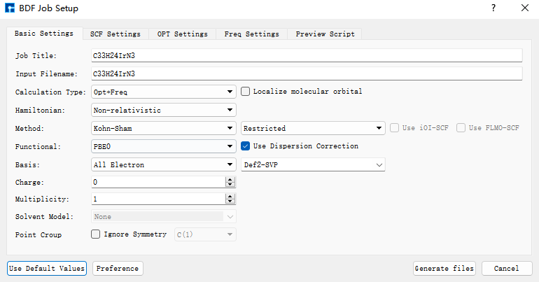
In the SCF Settings interface, select Coarse for DFT Integral Grid and Tight for Convergence Threshold. Use recommended default values for other parameters in the SCF Settings interface without modification.
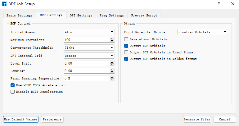
In the OPT Settings interface, select Tight for Convergence Threshold. Use recommended default values for other parameters in the OPT Settings interface without modification.
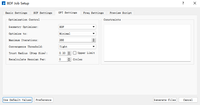
Use recommended default values for parameters in the Freq Settings interface without modification. Then click Generate files to generate the input file for the corresponding calculation. Select the generated bdf.inp file, right-click and choose open with to open the file, as shown below:
[File content unchanged - same as original]
Select the bdf.inp file, right-click and choose Run, the following server submission interface pops up:

Click Run to submit the job. After the job ends, three result files bdf.out, bdf.out.tmp, and bdf.scf.molden will appear in the Project.
Select bdf.out, right-click show view, in the Optimization dialog box, it shows that the structure has met the convergence criteria.
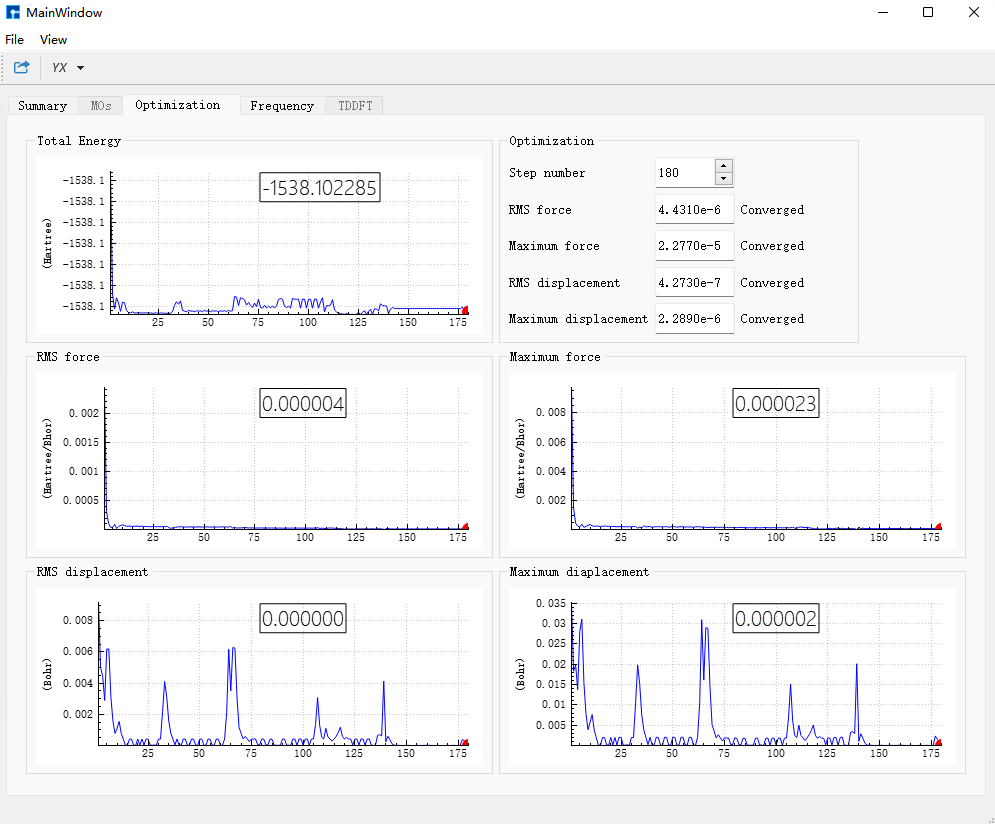
In the Frequency dialog box, check the frequencies; if no imaginary frequencies exist, it proves the structure has been optimized to a minimum point.
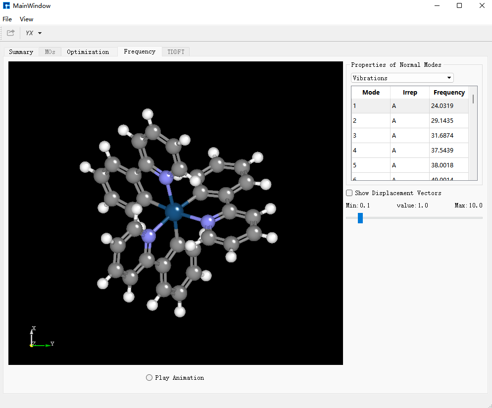
Excited State Optimization
Select the bdf.out file, right-click open with containing folder to open the folder. In the bdf.out file, search for converged in. The structure output under Molecular Cartesian Coordinates (X,Y,Z) in Angstrom : immediately following is the optimized S₀ structure of Ir(ppy)₃.
Save it as Irppy3_t1.xyz file, and drag Irppy3_t1.xyz into Device Studio for T₁ excited state structural optimization and frequency calculation.
Content of Irppy3_t1.xyz:
61

 Ir         -0.00021963       0.00084588       0.01424181
  C           2.59517396      -1.31710199      -0.58086411
  C           2.23709967       0.40664133      -2.11684705
  C           3.82729349      -1.60375453      -1.18851600
  C           2.03843393      -2.01080680       0.57861773
  C           3.44334868       0.17103124      -2.75937571
  H           1.56522101       1.20579483      -2.43942631
  C           4.25160770      -0.86138490      -2.27959559
  H           4.44860577      -2.40719663      -0.79331056
  C           2.69382363      -3.08153995       1.20802708
  H           3.74085930       0.78654308      -3.60925966
  H           5.21146469      -1.08097154      -2.75293386
  C           0.24421139      -2.16970311       2.17811922
  C           2.12763720      -3.69300459       2.31682204
  H           3.65478554      -3.44259873       0.83261331
  C           0.89831764      -3.22978876       2.79882363
  H          -0.71249803      -1.82386403       2.57651491
  H           2.63779958      -4.52517522       2.80699129
  H           0.44660698      -3.70582388       3.67403286
  C          -1.72035469       0.07933387       1.04722001
  C          -2.76313413      -0.76101290       0.56881686
  C          -2.01025266       0.87257612       2.17113445
  C          -4.02037491      -0.79383502       1.19368759
  C          -2.43582629      -1.59048558      -0.58889316
  C          -3.25751526       0.83538180       2.78746398
  H          -1.23410642       1.52839366       2.57249446
  C          -4.29332764       0.34509124       2.25152759
  H          -4.89835192      -1.11318656       0.80076906
  C          -3.29617560      -2.51740929      -1.19724703
  H          -3.44731484       1.46422538       3.66217358
  H          -5.27935386       0.39610056       2.71819787
  C          -0.75837785      -2.13799807      -2.04878703
  C          -3.02057249      -3.12865177      -2.21547404
  H          -4.44525951      -2.39959512      -0.77498376
  C          -1.70631730      -3.03592702      -2.67708276
  H           0.27022263      -1.95736074      -2.36320871
  H          -3.72428268      -3.82273458      -2.68079360
  H          -1.34337957      -3.64618311      -3.50492143
  N          -1.25281509      -1.36491844      -1.03498749
  C           0.05749757       2.91146589      -0.57266019
  C          -1.32777267       1.80183369      -2.13392316
  C          -0.20378718       4.13789922      -1.23242993
  C           0.84833732       2.74053836       0.60027468
  C          -1.62207961       2.97568834      -2.79963589
  H          -1.76529075       0.85235254      -2.45705604
  C          -1.02279372       4.18710974      -2.33345871
  H           0.25619858       5.05119986      -0.85064151
  C           0.99228869       1.37116718       1.10523883
  C           1.50408647       3.78492492       1.29091761
  H          -2.29824567       2.96275979      -3.65460398
  H          -1.21968527       5.13470890      -2.83803374
  C           1.79964051       1.14876808       2.23660071
  C           2.27478596       3.51131149       2.40946143
  H           1.40861651       4.81693356       0.94742301
  C           2.43450283       2.19478112       2.89597173
  H           1.90681895       0.12796182       2.60984200
  H           2.77105979       4.33756352       2.92655136
  H           3.04508360       2.00761950       3.78145403
  N          -0.50508694       1.73366277      -1.08285478
  N           1.77567220      -0.40171722      -1.08777429
  C           0.72548984      -1.57229627       1.07484739
Select Simulator → BDF → BDF, set parameters in the interface. In the Basic Settings interface, select TDDFT-OPT+Freq for Calculation Type, use the default PBE0 functional for method, and select Def2-SVP basis set under All Electron type in Basis. Use recommended default values for other parameters in the Basic Settings interface without modification.
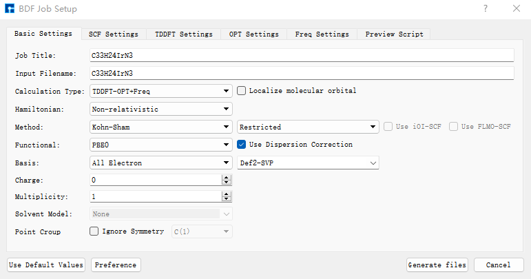
In the SCF Settings interface, uncheck the default Use MPEC+COSX Acceleration. Use recommended default values for other parameters in the SCF Settings interface without modification.
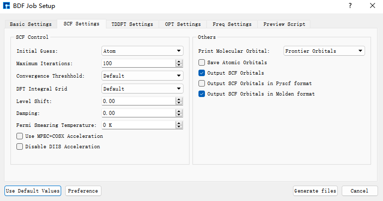
In the TDDFT Settings panel, uncheck the default Use MPEC+COSX Acceleration. Select Triplet for Multiplicity and Very Tight for Convergence Threshold. Use recommended default values for other parameters in the TDDFT Settings interface without modification.
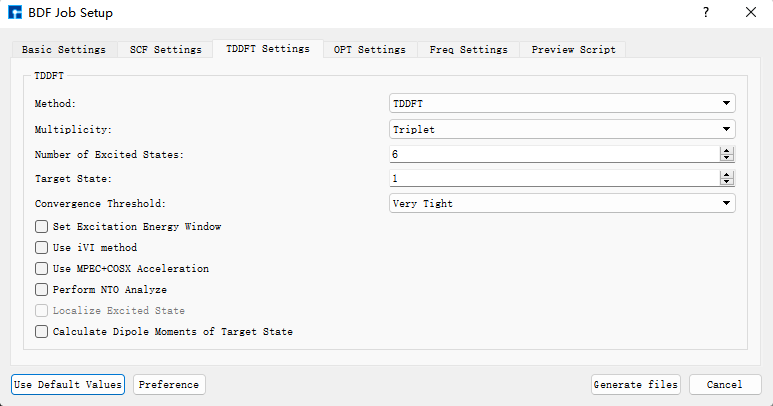
Use recommended default values for parameters in the OPT Settings and Freq Settings panels without modification. Then click Generate files to generate the input file for the corresponding calculation. Select the generated bdf.inp file, right-click and choose open containing folder to enter the folder. In the bdf.inp’s $tddft module, add:
Gridtol
1E-6
Content of bdf.inp:
[File content unchanged - same as original]
Select the bdf.inp file, right-click and choose Run to submit the job. After the job ends, three result files bdf.out, bdf.out.tmp, and bdf.scf.molden will appear in the Project.
Select bdf.out, right-click show view, in the Optimization dialog box, it shows that the structure has met the convergence criteria.
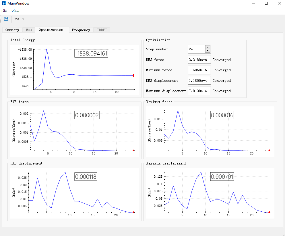
In the Frequency dialog box, check the frequencies; if no imaginary frequencies exist, it proves the structure has been optimized to a minimum point.
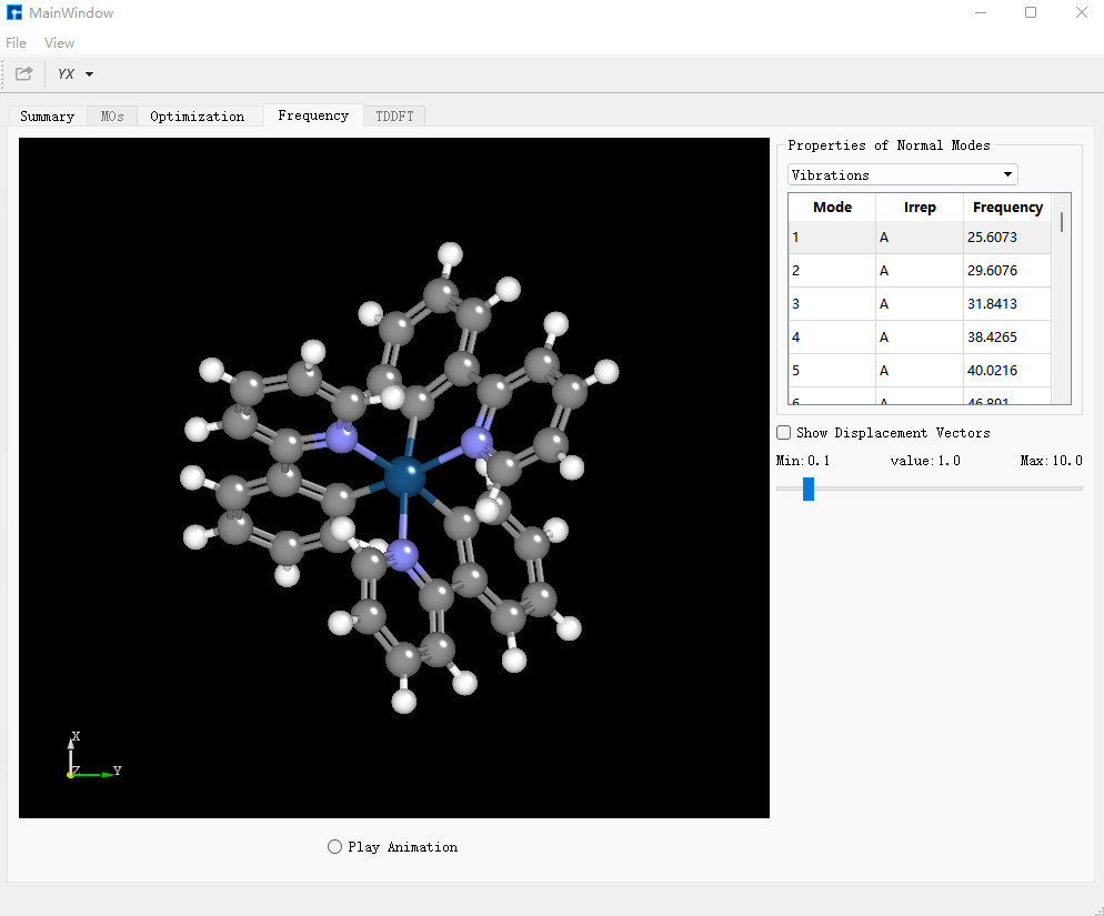
Spin-Orbit Coupling
Select the bdf.out file, right-click open with containing folder to open the bdf.out file. In the file, search for converged in. The structure output under Molecular Cartesian Coordinates (X,Y,Z) in Angstrom : immediately following is the optimized T₁ excited state structure. Save it as Irppy3_t1_soc.xyz file:
61

  Ir          0.00713728       0.02772384       0.06844143
  C           2.49525480      -1.44901550      -0.61634342
  C           2.18832036       0.30085414      -2.14613716
  C           3.68634391      -1.80881598      -1.26572189
  C           1.93194560      -2.11689508       0.55823360
  C           3.35838993      -0.00562745      -2.82371008
  H           1.54555778       1.13535499      -2.43828057
  C           4.11644204      -1.08671357      -2.36826138
  H           4.27131595      -2.65056635      -0.89578008
  C           2.53568350      -3.23676194       1.15281696
  H           3.66807720       0.59265321      -3.68133338
  H           5.04582829      -1.36185464      -2.87261245
  C           0.15985754      -2.20796739       2.19060975
  C           1.95468524      -3.83725789       2.26057143
  H           3.46642195      -3.64596143       0.75209976
  C           0.76249168      -3.31842903       2.77624738
  H          -0.76777546      -1.81381956       2.61329026
  H           2.42616559      -4.70662836       2.72403491
  H           0.30108846      -3.78788395       3.64972556
  C          -1.72817262       0.21988877       1.05055833
  C          -2.80684294      -0.57231379       0.57552059
  C          -1.98377974       1.07446425       2.13652018
  C          -4.07348284      -0.50293868       1.17614116
  C          -2.51722058      -1.44616477      -0.55935718
  C          -3.24105830       1.13344573       2.72846833
  H          -1.17254968       1.69178400       2.52835606
  C          -4.29332764       0.34509124       2.25152759
  H          -4.89835192      -1.11318656       0.80076906
  C          -3.42583031      -2.33456216      -1.15446766
  H          -3.44731484       1.80444609       3.66217358
  H          -5.27935386       0.39610056       2.71819787
  C          -0.85701735      -2.13799807      -2.04878703
  C          -3.02057249      -3.12865177      -2.21547404
  H          -4.44525951      -2.39959512      -0.77498376
  C          -1.70631730      -3.03592702      -2.67708276
  H           0.18295061      -1.95736074      -2.36320871
  H          -3.72428268      -3.82273458      -2.68079360
  H          -1.34337957      -3.64618311      -3.50492143
  N          -1.25281509      -1.36491844      -1.03498749
  C           0.05749757       2.91146589      -0.57266019
  C          -1.32777267       1.80183369      -2.13392316
  C          -0.20378718       4.13789922      -1.23242993
  C           0.84833732       2.74053836       0.60027468
  C          -1.62207961       2.97568834      -2.79963589
  H          -1.76529075       0.85235254      -2.45705604
  C          -1.02279372       4.18710974      -2.33345871
  H           0.25619858       5.05119986      -0.85064151
  C           0.99228869       1.37116718       1.10523883
  C           1.50408647       3.78492492       1.29091761
  H          -2.29824567       2.96275979      -3.65460398
  H          -1.21968527       5.13470890      -2.83803374
  C           1.79964051       1.14876808       2.23660071
  C           2.27478596       3.51131149       2.40946143
  H           1.40861651       4.81693356       0.94742301
  C           2.43450283       2.19478112       2.89597173
  H           1.90681895       0.12796182       2.60984200
  H           2.77105979       4.33756351       2.92655136
  H           3.04508360       2.00761950       3.78145403
  N          -0.50508694       1.73366277      -1.08285478
  N           1.77567220      -0.40171722      -1.08777429
  C           0.72548984      -1.57229627       1.07484739
Based on the T₁ excited state structure, perform spin-orbit coupling (SOC) calculation between S₀ and T₁. Drag Irppy3_t1_soc.xyz into Device Studio, select Simulator → BDF → BDF, set parameters in the interface. In the Basic Settings interface, select TDDFT-SOC for Calculation Type, choose PBE0 for Functional, uncheck Use Dispersion Correction. Select sf-X2C for Hamiltonian, and choose x2c-SVPall basis set under All Electron type in Basis.
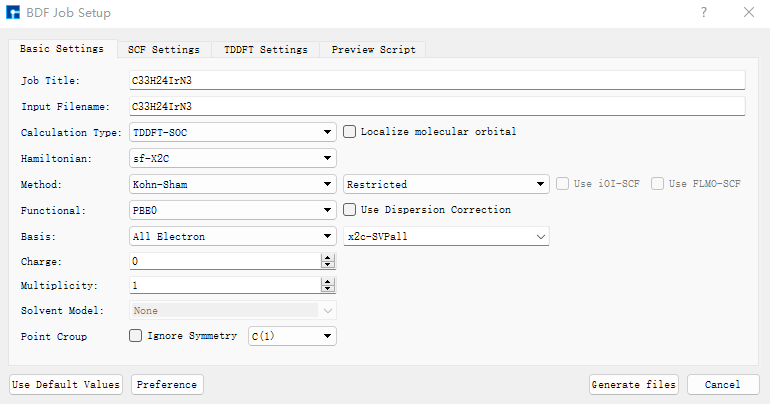
In the TDDFT Settings panel, check “Including Ground State” in the Spin-Orbit Coupling section.
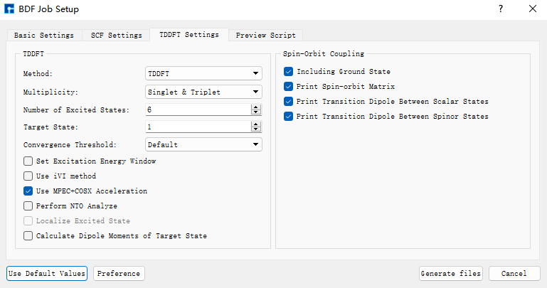
Use recommended default values for other parameters in Basic Settings, SCF Settings, and TDDFT Settings without modification. Then click Generate files to create the corresponding input file. Select the generated bdf.inp file, right-click and choose open with to open it as shown below:
The generated input file bdf.inp is:
[File content unchanged - same as original]
Select the bdf.inp file, right-click and choose Run to submit the job. After the job completes, the result files bdf.out and bdf.scf.molden will appear in the Project. Select bdf.out, right-click and choose show view. In the TDDFT panel, select Spinor, and identify the 2nd, 3rd, and 4th states as the three components of T₁ in Dominant Excitations.
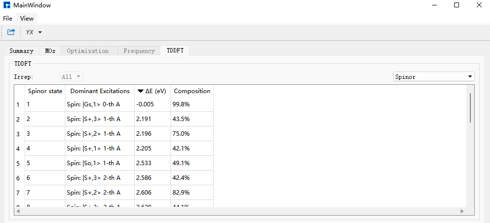
Click the bdf.out file, right-click and choose Open Containing Folder to enter the folder. Open bdf.out, search for *** List of SOC-SI results ***, and read the ExEnergies for states 2, 3, and 4 as: 2.1906 eV, 2.1961 eV, and 2.2052 eV respectively.
*** List of SOC-SI results ***

No.      ExEnergies            Dominant Excitations         Esf        dE      Eex(eV)     (cm^-1)

  1      -0.0054 eV    99.8%  Spin: |Gs,1>    0-th    A    0.0000   -0.0054    0.0000         0.00
  2       2.1906 eV    43.5%  Spin: |S+,3>    1-th    A    2.2232   -0.0326    2.1961     17712.45
  3       2.1961 eV    75.0%  Spin: |S+,2>    1-th    A    2.2232   -0.0272    2.2015     17756.09
  4       2.2052 eV    42.1%  Spin: |S+,1>    1-th    A    2.2232   -0.0180    2.2106     17829.67
  5       2.5334 eV    49.1%  Spin: |So,1>    1-th    A    2.6854   -0.1520    2.5388     20477.15
  6       2.5861 eV    42.4%  Spin: |S+,3>    2-th    A    2.6312   -0.0452    2.5915     20901.71
  7       2.6064 eV    82.9%  Spin: |S+,2>    2-th    A    2.6312   -0.0248    2.6118     21065.69
Search for E_tot and read the corresponding energy as -19265.29575859. The energies of the three sub-states of T₁ are obtained by adding E_tot and ExEnergies energies. For the second sub-state (state 2), the calculation is: -19265.29575859 + 2.1906/27.2114 = -19265.215256 au. The energy of the third sub-state is -19265.215053 au. The energy of the fourth sub-state is -19265.214719 au.
 Final scf result
 E_tot =            -19265.29575859
 E_ele =            -25841.98940694
 E_nn  =              6576.69364834
 E_1e  =            -39510.05277256
 E_ne  =            -66428.66809936
 E_kin =             26918.61532681
 E_ee  =             14091.21945939
 E_xc  =              -423.15609377
Virial Theorem      1.715687
Using the same method and basis set, calculate SOC for the S₀ ground state structure. In bdf.out, search for E_tot and read the corresponding energy as: -19265.30415493 au.
 Final scf result
 E_tot =            -19265.30415493
 E_ele =            -25838.09048037
 E_nn  =              6572.78632544
 E_1e  =            -39502.28526599
 E_ne  =            -66421.04136762
 E_kin =             26918.75610162
 E_ee  =             14087.38176801
 E_xc  =              -423.18698239
Virial Theorem      1.715683
The energies of the three T₁ sub-states relative to S₀ are obtained by subtracting the S₀ state energy from the three sub-state energies: 0.088899 au, 0.089102 au, and 0.089436 au respectively. In the SOC calculation output file for the T₁ structure, search for [tddft_soc_matrso]:, which outputs the energies and transition dipole moments of each excited state relative to the ground state after considering SOC.
    [tddft_soc_matrso]: Print selected matrix elements of [dpl]

 No.  ( I , J )   |rij|^2       E_J-E_I         fosc          rate(s^-1)
-------------------------------------------------------------------------------
  1     1    2   0.104E-02    2.196064924    0.000056149     0.117E+05
  Details of transition dipole moment with SOC (in a.u.):
                  <I|X|J>       <I|Y|J>       <I|Z|J>        (also in debye)
         Real=   0.279E-01     0.161E-01    -0.216E-02     0.0710   0.0409  -0.0055
         Imag=   0.123E-07    -0.291E-07    -0.867E-08     0.0000  -0.0000  -0.0000
         Norm=   0.279E-01     0.161E-01     0.216E-02

 No.  ( I , J )   |rij|^2       E_J-E_I         fosc          rate(s^-1)
-------------------------------------------------------------------------------
  2     1    3   0.354E-03    2.201474871    0.000019090     0.401E+04
  Details of transition dipole moment with SOC (in a.u.):
                  <I|X|J>       <I|Y|J>       <I|Z|J>        (also in debye)
         Real=   0.587E-02     0.179E-01     0.126E-03     0.0149   0.0454   0.0003
         Imag=  -0.108E-06    -0.357E-07     0.361E-07    -0.0000  -0.0000   0.0000
         Norm=   0.587E-02     0.179E-01     0.126E-03

 No.  ( I , J )   |rij|^2       E_J-E_I         fosc          rate(s^-1)
-------------------------------------------------------------------------------
  3     1    4   0.259E-01    2.210597826    0.001400915     0.297E+06
  Details of transition dipole moment with SOC (in a.u.):
                  <I|X|J>       <I|Y|J>       <I|Z|J>        (also in debye)
         Real=   0.905E-08    -0.356E-07    -0.418E-08     0.0000  -0.0000  -0.0000
         Imag=  -0.535E-01     0.148E+00     0.316E-01    -0.1360   0.3771   0.0802
         Norm=   0.535E-01     0.148E+00     0.316E-01

 No.  ( I , J )   |rij|^2       E_J-E_I         fosc          rate(s^-1)
-------------------------------------------------------------------------------
  4     1    5   0.154E+00    2.538843563    0.009594212     0.268E+07
  Details of transition dipole moment with SOC (in a.u.):
                  <I|X|J>       <I|Y|J>       <I|Z|J>        (also in debye)
         Real=  -0.236E+00     0.158E+00     0.271E+00    -0.5998   0.4010   0.6899
         Imag=  -0.271E-06     0.183E-06     0.310E-06    -0.0000   0.0000   0.0000
         Norm=   0.236E+00     0.158E+00     0.271E+00

 No.  ( I , J )   |rij|^2       E_J-E_I         fosc          rate(s^-1)
-------------------------------------------------------------------------------
  5     1    6   0.275E-02    2.591483156    0.000174312     0.508E+05
  Details of transition dipole moment with SOC (in a.u.):
                  <I|X|J>       <I|Y|J>       <I|Z|J>        (also in debye)
         Real=   0.339E-01     0.292E-01     0.273E-01     0.0861   0.0743   0.0693
         Imag=  -0.132E-07     0.447E-07     0.428E-07    -0.0000   0.0000   0.0000
         Norm=   0.339E-01     0.292E-01     0.273E-01
Here, 1 2 represents the transition dipole moment between the first and second spinor states, and so on. We need the excitation energies and transition dipole moments for the 1st, 2nd, and 3rd excited states.
The transition dipole moment data is listed in Details of transition dipole moment with SOC (in a.u.):. The first three columns are dipole moments in atomic units (au), and the next three columns are in Debye.
To obtain the transition dipole moment for each state, take the square root of the sum of squares of the six numbers in Debye units. Alternatively, take the square root of the sum of squares of the three Norm values and multiply by 2.5417. This gives transition dipole moments of 0.082058 Debye, 0.047881 Debye, and 0.407979 Debye for the 1st, 2nd, and 3rd excited states respectively.
These six parameters will be used in MOMAP software for phosphorescence emission rate calculations.
At this point, all necessary files and parameters for MOMAP’s phosphorescence radiative rate calculation for \(\rm Ir(ppy)_3\) are complete, including BDF’s structural optimization frequency result files, spin-orbit coupling calculation result files, and parameters.
Phosphorescence Radiative Rate
Next, we begin calculating the phosphorescence radiative rate of \(\rm Ir(ppy)_3\) using MOMAP.
First, to calculate the T₁→S₀ phosphorescence radiative rate, start with electron-vibration coupling (EVC) calculation. This calculation is based on molecular vibration frequencies and force constant matrices output from quantum calculations. It computes mode displacements, Huang-Rhys factors, reorganization energies, and Duschinsky rotation matrices between initial and final states of molecular transitions in both internal and Cartesian coordinates.
Rename the optimized frequency calculation files for \(\rm Ir(ppy)_3\)’s ground state from BDF to irppy3_s0.out, and the T₁ optimized frequency calculation file to irppy3_t1.out. Place both in the EVC calculation folder.
The input file for EVC calculation momap.inp is:
do_evc=1

&evc
        ffreq(1)="irppy3_s0.out"
        ffreq(2)="irppy3_t1.out"
        proj_reorg=.t.
/
Submit the script file momap.slurm to run the job. After successful completion, use evc.cart.dat for subsequent T₁→S₀ phosphorescence emission rate calculations. Perform calculations for each of T₁’s three states. For the first sub-state (state 2), the input file momap.inp is:
do_spec_tvcf_ft   = 1
do_spec_tvcf_spec = 1

&spec_tvcf
  DUSHIN        = .t.
  Temp          = 300 K
  tmax          = 1000 fs
  dt            = 1   fs
  Ead           = 0.088899 au
  EDMA          = 1 debye
  EDME          = 0.082058 debye
  FreqScale     = 1
  DSFile        = "evc.cart.dat"
  Emax          = 0.3 au
  dE            = 0.00001 au
  logFile       = "spec.tvcf.log"
  FtFile        = "spec.tvcf.ft.dat"
  FoFile        = "spec.tvcf.fo.dat"
  FoSFile       = "spec.tvcf.spec.dat"
/
Submit the script file momap.slurm to run the job. After completion, verify if the correlation function converges.
Open spec.tvcf.log. The phosphorescence radiative rate is read from the first and second numbers, in a.u. and s⁻¹ units respectively. The third number is the lifetime in ns.
For the second sub-state (state 3), the input file momap.inp is:
do_spec_tvcf_ft   = 1
do_spec_tvcf_spec = 1

&spec_tvcf
  DUSHIN        = .t.
  Temp          = 300 K
  tmax          = 1000 fs
  dt            = 1   fs
  Ead           = 0.089102 au
  EDMA          = 1 debye
  EDME          = 0.047881 debye
  FreqScale     = 1
  DSFile        = "evc.cart.dat"
  Emax          = 0.3 au
  dE            = 0.00001 au
  logFile       = "spec.tvcf.log"
  FtFile        = "spec.tvcf.ft.dat"
  FoFile        = "spec.tvcf.fo.dat"
  FoSFile       = "spec.tvcf.spec.dat"
/
Submit the script file momap.slurm to run the job.
For the third sub-state (state 4), the input file momap.inp is:
do_spec_tvcf_ft   = 1
do_spec_tvcf_spec = 1

&spec_tvcf
  DUSHIN        = .t.
  Temp          = 300 K
  tmax          = 1000 fs
  dt            = 1   fs
  Ead           = 0.089436 au
  EDMA          = 1 debye
  EDME          = 0.407979 debye
  FreqScale     = 1
  DSFile        = "evc.cart.dat"
  Emax          = 0.3 au
  dE            = 0.00001 au
  logFile       = "spec.tvcf.log"
  FtFile        = "spec.tvcf.ft.dat"
  FoFile        = "spec.tvcf.fo.dat"
  FoSFile       = "spec.tvcf.spec.dat"
/
Finally, weight the phosphorescence emission rates of the three sub-states according to their Boltzmann distribution based on relative energies (refer to http://sobereva.com/462 and http://sobereva.com/165 for details and corresponding Excel templates). Sum them to obtain the final T₁ state phosphorescence emission rate.
Quantum Theoretical Study of the Anti-Kasha Rule Fluorescence Mechanism in Azulene
According to Kasha’s rule, molecular fluorescence or phosphorescence originates from the lowest singlet or triplet state due to rapid non-radiative transitions between higher excited states. Azulene is a classic example that violates Kasha’s rule. The fluorescence of azulene originates from the S₂ state, which can be attributed to the large energy gap between S₂→S₁ that reduces the S₂→S₁ internal conversion rate. Additionally, the relatively small energy gap between S₁ and S₀ results in a high internal conversion rate, thereby reducing the fluorescence quantum efficiency of S₁→S₀, making S₁→S₀ fluorescence difficult to observe. Here, using the BDF and MOMAP software, we calculate the radiative rate and internal conversion rate of azulene’s S₁→S₀ transition to explain the experimental observation that the extremely low quantum efficiency of azulene’s first excited state makes its fluorescence difficult to detect.
The MOMAP calculation for azulene’s S₁→S₀ radiative rate and internal conversion rate requires the structural optimization frequency results file, non-adiabatic coupling results file, and parameters from the BDF quantum software. First, we complete the BDF calculation part.
BDF Calculation Part
Prepare the xyz file of azulene’s molecular structure:
18

C                 -0.48100000    0.74480000    0.00000000
C                 -0.56240000   -0.71320000    0.00020000
C                 -1.75790000    1.17860000   -0.00030000
C                 -1.96510000   -1.08880000    0.00000000
C                  0.66870000    1.60890000    0.00030000
C                  0.45100000   -1.58850000    0.00030000
C                 -2.66930000    0.05180000   -0.00010000
C                  1.95140000    1.22210000    0.00020000
C                  1.86730000   -1.29960000   -0.00020000
C                  2.49720000   -0.11610000   -0.00040000
H                 -2.09080000    2.20560000   -0.00040000
H                 -2.35750000   -2.09240000    0.00010000
H                  0.46620000    2.67860000    0.00070000
H                  0.22090000   -2.65340000    0.00040000
H                 -3.74370000    0.14050000   -0.00030000
H                  2.70720000    2.00650000    0.00050000
H                  2.49320000   -2.19150000   -0.00060000
H                  3.58670000   -0.13930000   -0.00080000
Open Device Studio, click File → New Project, name it fluorescence.hpf, drag azulene.xyz into the Project, and double-click azulene.hzw to get the interface shown below.
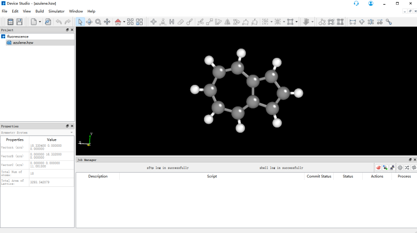
First, perform structural optimization and frequency calculation of azulene using BDF. Select Simulator → BDF → BDF, set parameters in the interface. In the Basic Settings interface, select Opt+Freq for Calculation Type, use the default GB3LYP functional for method, and select 6-31G(d,p) for basis set under All Electron type in Basis. Other parameters in the Basic Settings interface and parameters in panels like SCF Settings, OPT Settings, Freq Settings use recommended default values without modification. Then click Generate files to generate the input file for the corresponding calculation.
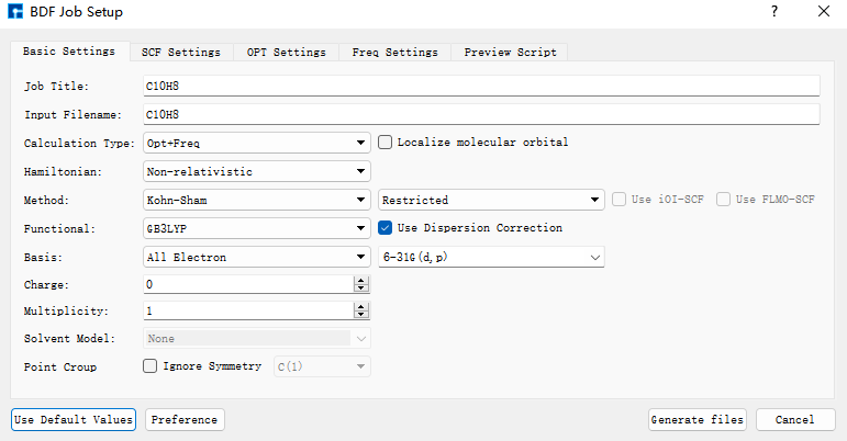
Select the generated bdf.inp file, right-click and choose open with to open the file, as shown below:
[File content unchanged - same as original]
Select the bdf.inp file, right-click and choose Run, the following interface pops up:
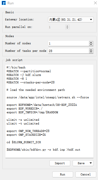
Click Run to submit the job, and the real-time output of the result file will automatically pop up.
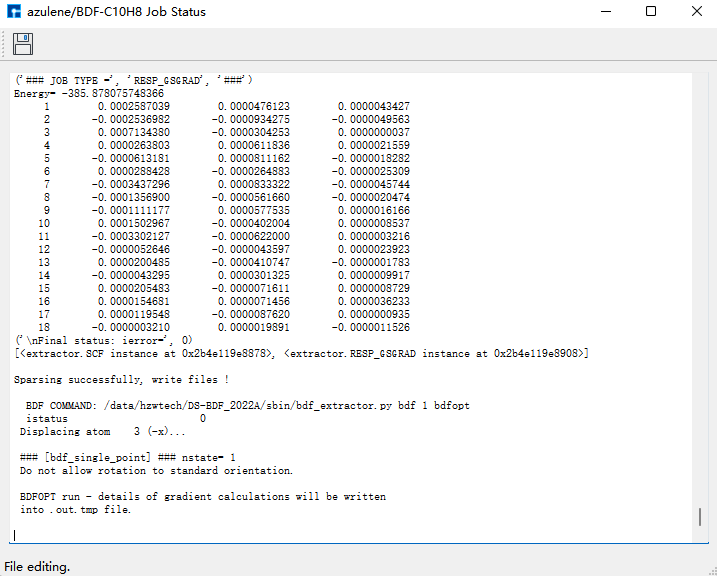
After the job ends, three result files bdf.out, bdf.out.tmp, and bdf.scf.molden will appear in the Project.
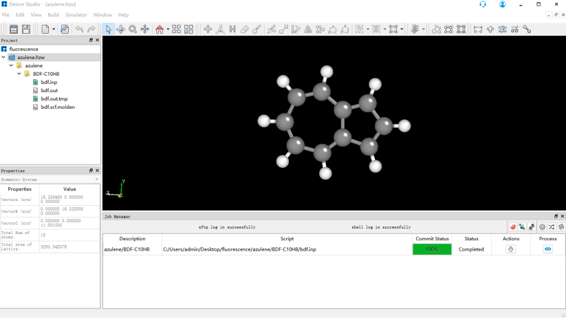
Select bdf.out, right-click show view, in the Optimization dialog box, it shows that the structure has met the convergence criteria.
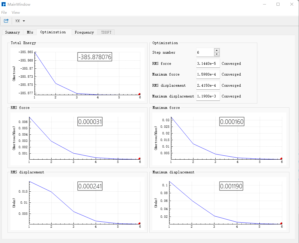
In the Frequency dialog box, check the frequencies; if no imaginary frequencies exist, it proves the structure has been optimized to a minimum point.
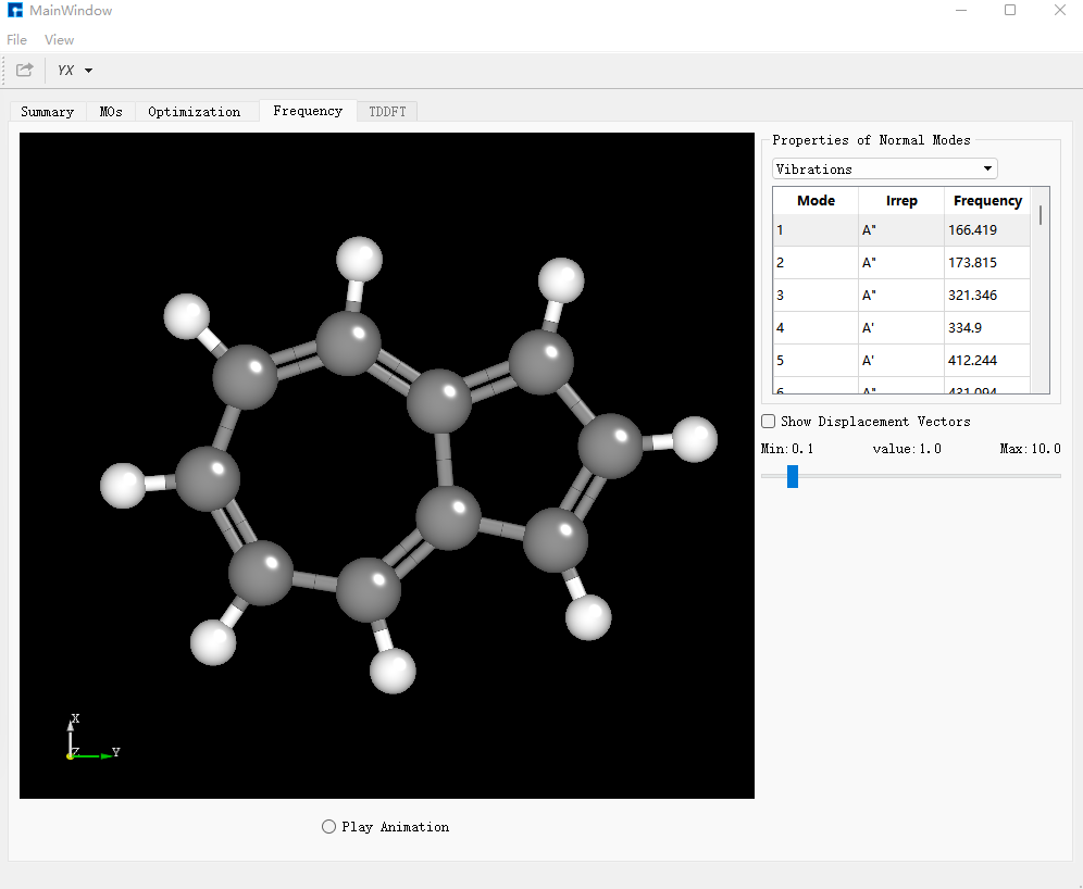
In the Summary dialog box, Total Energy is -385.87807600 a.u., which is the required single-point energy of the ground state azulene.
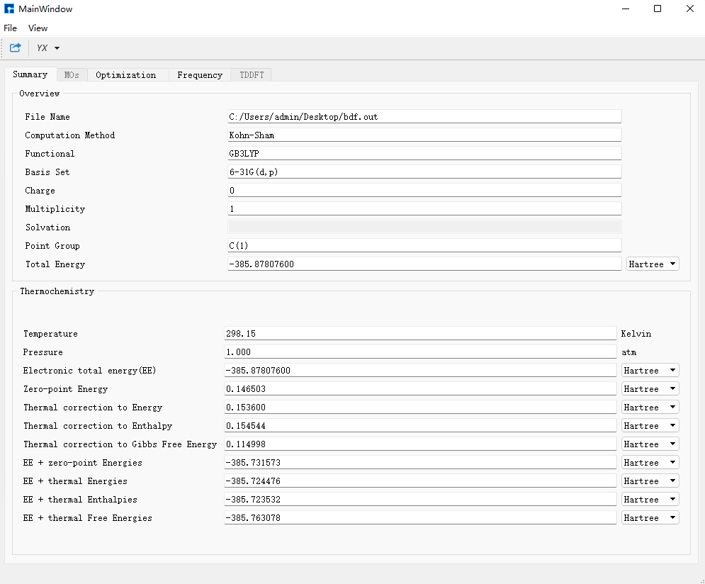
Click the calculation task in Job Manager, click the server, which has entered the folder where the task is located, enter /data/hzwtech/DS-BDF_2022A/sbin/optgeom2xyz.py bdf.optgeom, press Enter to generate the bdf.xyz file. Click the file transfer tool, enter the folder, drag out the bdf.xyz file, which is the input file needed for the next excited state structure optimization. Rename it to azulene_s0.xyz, open the folder, remove the second line of description, and drag it into Device Studio.
Perform S₁ excited state structure optimization and frequency calculation of azulene using BDF. Select Simulator → BDF → BDF, set parameters in the interface. In the Basic Settings interface, select TDDFT-OPT+Freq for Calculation Type, use the default GB3LYP functional for method, and select 6-31G(d,p) for basis set under All Electron type in Basis. In SCF Settings and TDDFT Settings panels, uncheck the default Use MPEC+COSX Acceleration. Other parameters in Basic Settings, SCF Settings, TDDFT Settings interfaces and parameters in panels like OPT Settings, Freq Settings use recommended default values without modification. Then click Generate files to generate the input file for the corresponding calculation.
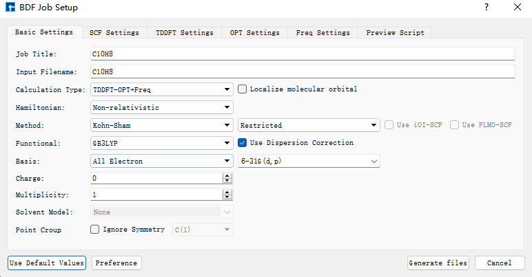
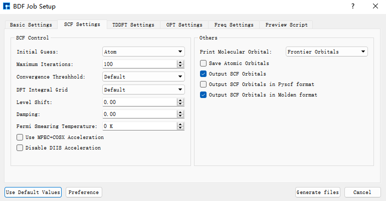
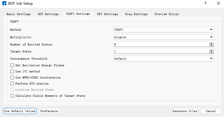
Select the generated bdf.inp file, right-click and choose open with to open the file, as shown below:
[File content unchanged - same as original]
Select the bdf.inp file, right-click and choose Run to submit the job. After the job ends, three result files bdf.out, bdf.out.tmp, and bdf.scm.molden will appear in the Project.
Select bdf.out, right-click show view, in the Optimization dialog box, it shows that the structure has met the convergence criteria.
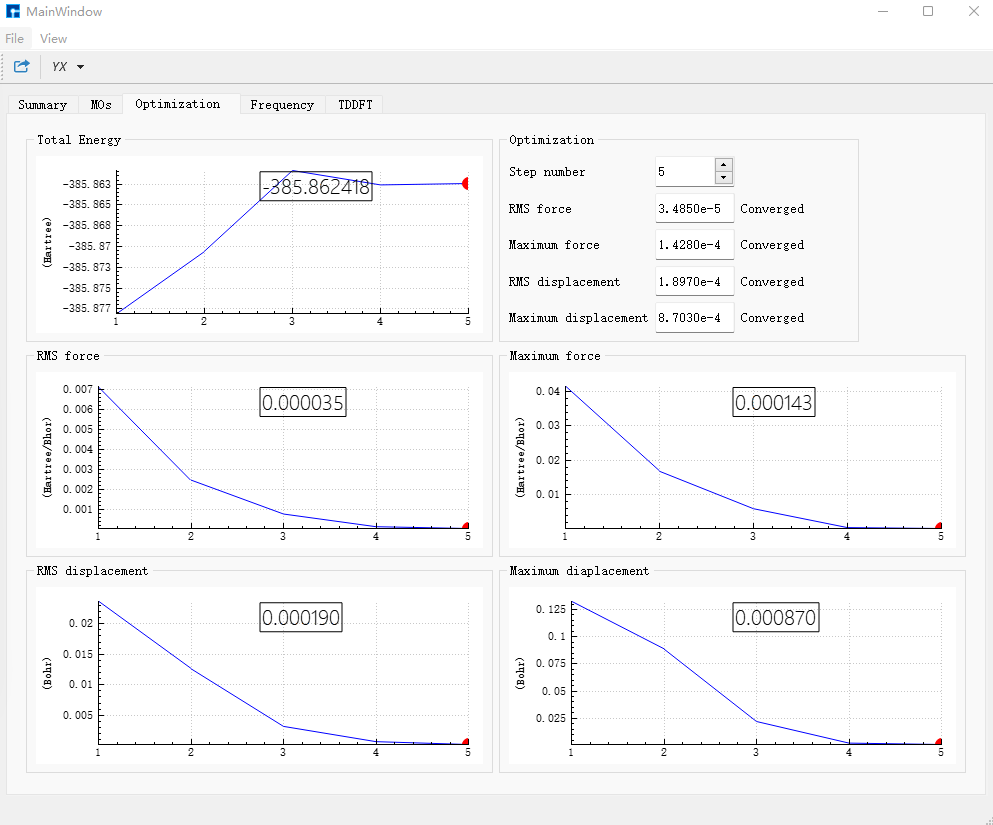
In the Frequency dialog box, check the frequencies; if no imaginary frequencies exist, it proves the structure has been optimized to a minimum point.
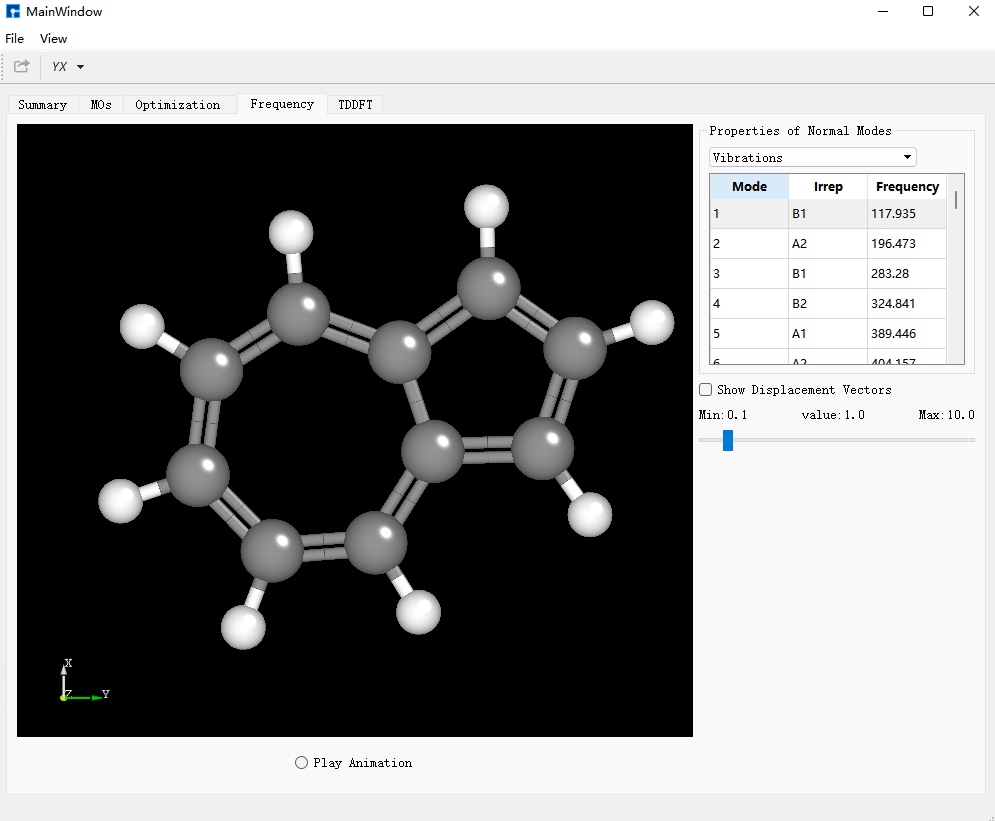
Select bdf.out.tmp, right-click open with containing folder, open bdf.out.tmp, and find the first tddft calculation module module tddft at the beginning of the file. According to the Ground to excited state Transition electric dipole moments (Au) in the tddft module, get the EDMA parameter needed by MOMAP from State 1’s transition electric dipole moment. Calculation method: \(\sqrt{(0.3456)^2+(-0.1159)^2+(-0.0000)^2} = 0.3646\) a.u. Convert units from a.u. to Debye: EDMA = 0.3646 * 2.5417 = 0.9267 Debye.
[File content unchanged - same as original]
At the end of the file, find the first tddft calculation module module tddft. According to the Ground to excited state Transition electric dipole moments (Au) in the tddft module, get the EDME parameter needed by MOMAP from State 1’s transition electric dipole moment. Calculation method: \(\sqrt{(-0.2427)^2+(0.0816)^2+(-0.0000)^2} = 0.2560\) a.u. Convert units from a.u. to Debye: EDME = 0.2560 * 2.5417 = 0.6507 Debye.
[File content unchanged - same as original]
In this tddft module’s Statistics for [dvdson_rpa_block]:, read the energy of state No. 1 as -385.8030480568 a.u., which is the single-point energy of S₁ state.
[File content unchanged - same as original]
Subtract the S₁ state’s single-point energy from S₀ state’s single-point energy to get the energy difference parameter Ead = 0.07502 a.u. needed by MOMAP.
Based on the ground state structure, perform non-adiabatic coupling calculation between S₀ and S₁. Click azulene_s0.hzw, right-click and click copy, set new file name to nacme, and nacme.hzw appears in the Project. Double-click nacme.hzw, use BDF to perform azulene’s non-adiabatic coupling calculation. Select Simulator → BDF → BDF, set parameters in the interface. In the Basic Settings interface, select TDDFT-NAC for Calculation Type, use the default GB3LYP functional for method, and select 6-31G(d,p) for basis set under All Electron type in Basis. In SCF Settings and TDDFT Settings panels, uncheck the default Use MPEC+COSX Acceleration. In the Non-Adiabatic Coupling content box in the TDDFT Settings panel, under the default Coupling between Ground and Excited-State, click the “+” sign. Other parameters in Basic Settings, SCF Settings, TDDFT Settings interfaces and parameters in panels like OPT Settings, Freq Settings use recommended default values without modification. Then click Generate files to generate the input file for the corresponding calculation.
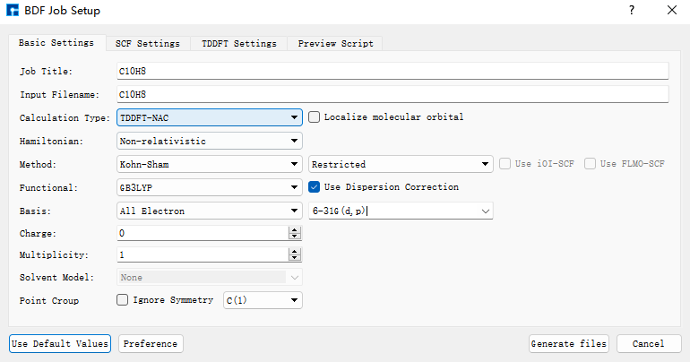
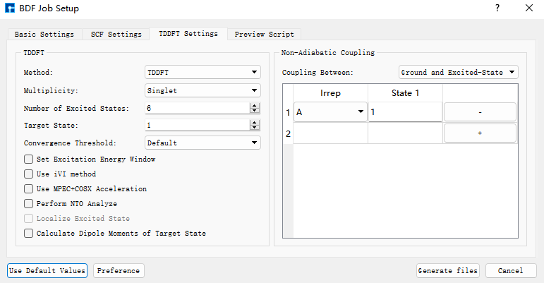
Select the generated bdf.inp file, right-click and choose open with to open the file, as shown below:
[File content unchanged - same as original]
Select the bdf.inp file, right-click and choose Run to submit the job. After the job ends, two result files bdf.out and bdf.scf.molden will appear in the Project.
At this point, the BDF quantum software calculation part required for MOMAP’s calculation of azulene’s S₁→S₀ radiative rate and internal conversion rate—including structural optimization frequency result files, non-adiabatic coupling result files, and parameter parts—are all completed.
MOMAP Calculation Part
After completing the structural optimization, frequency calculation, and non-adiabatic coupling calculation of azulene using BDF quantum software and calculating the parameters needed in the MOMAP input file, we will use MOMAP software to calculate the radiative rate and internal conversion rate of azulene’s S₁→S₀ transition. By comparing the radiative rate and internal conversion rate, we explain why azulene’s S₁→S₀ fluorescence is difficult to observe.
First, calculate the fluorescence radiative rate of S₁→S₀. The first step is to perform electron-vibration coupling (EVC) calculation. This calculation is based on the molecular vibration frequencies and force constant matrices output from quantum calculations, and computes the mode displacement, Huang-Rhys factor, reorganization energy, and Duschinsky rotation matrix between the initial and final states of molecular transitions in both internal and Cartesian coordinates.
Rename BDF’s S₀ optimization frequency calculation result to azulene-s0.out and S₁ calculation result to azulene-s1.out, and place them in the EVC calculation folder. The input file momap.inp for EVC calculation is:
do_evc          = 1

&evc
  ffreq(1)      = "azulene-s0.out"
  ffreq(2)      = "azulene-s1.out"
  proj_reorg = .t.
/
Submit the script file momap.slurm. After the job runs, the following files are generated:
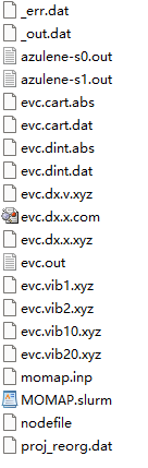
evc.cart.dat contains the results of mode displacement, Huang-Rhys factor, reorganization energy, and Duschinsky rotation matrix calculated using Cartesian coordinates; while evc.dint.dat contains results of mode displacement and Huang-Rhys factor calculated using internal coordinates, and reorganization energy and Duschinsky rotation matrix calculated using Cartesian coordinates.
Open the evc.cart.dat file to view the total reorganization energy value:
--------------------------------------------------------------------------------------------------------------------------------------------
  Total reorganization energy      (cm-1):         4032.869339       5126.265767
--------------------------------------------------------------------------------------------------------------------------------------------
Compare with the value in the evc.dint.dat file:
--------------------------------------------------------------------------------------------------------------------------------------------
  Total reorganization energy      (cm-1):         4070.407661       5114.173064
--------------------------------------------------------------------------------------------------------------------------------------------
Compare the reorganization energies in the evc.cart.dat and evc.dint.dat files. If the reorganization energies are not significantly different (< \(1000 cm^{-1}\)), use the evc.cart.dat file for subsequent calculations. If they differ significantly (generally evc.cart.dat > evc.dint.dat), use the evc.dint.dat file. Here they are relatively close and reasonable (< \(10000 cm^{-1}\)), so we use evc.cart.dat for the next step of S₁→S₀ fluorescence radiative rate calculation.
Additionally, more post-processing can be done based on the EVC calculation result files.
evc.dx.x.com and evc.dx.x.xyz are molecular superposition diagrams of the two electronic states. evc.dx.x.com can be opened with GaussView. Select Tube type under View → Display Format → Molecule, displayed as:
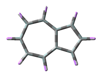
evc.dx.x.xyz can be opened with Jmol software, displayed as:
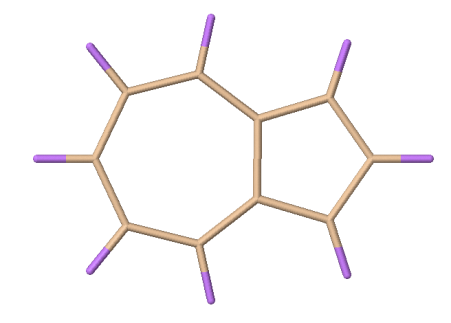
evc.dx.v.xyz is also a molecular state superposition diagram. Open it with Jmol software, select Display → Vector → 0.1A, displayed as:
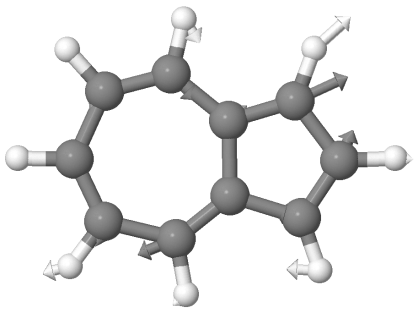
evc.cart.abs is the Duschinsky matrix file, which can be used to plot the Duschinsky matrix 2D diagram. In Device Studio, select Simulator → momap → analysis, open the evc.cart.abs file, displayed as:
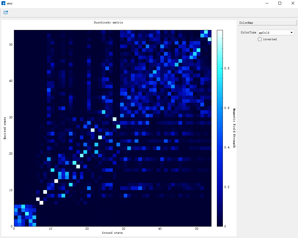
Similarly, open the evc.dint.abs file. You can select the display color in the ColorType drop-down box, displayed as:
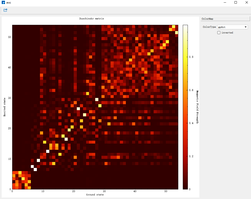
Both Duschinsky matrices are calculated using Cartesian coordinates—choose either.
Place the evc.vib1.xyz and evc.vib2.xyz files in the same path as the evc.cart.dat file. In Device Studio, select Simulator → momap → analysis, open the evc.cart.dat file, and diagrams of reorganization energy and Huang-Rhys factors corresponding to each vibration mode in ground and excited states appear, displayed as:
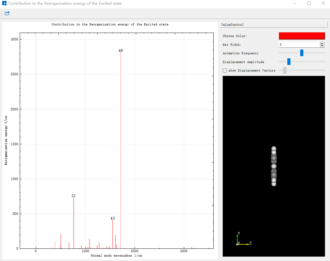
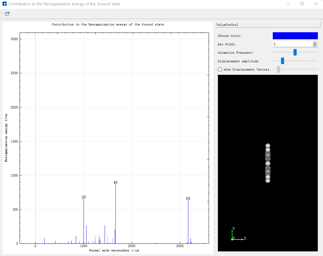
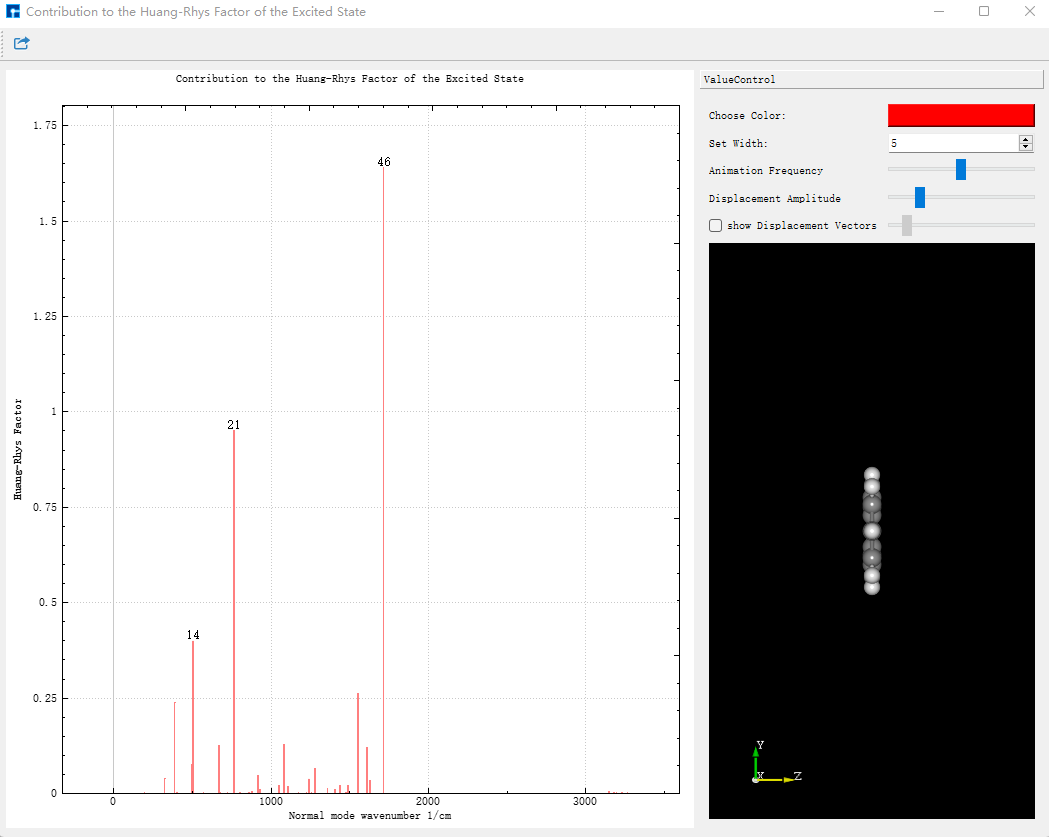
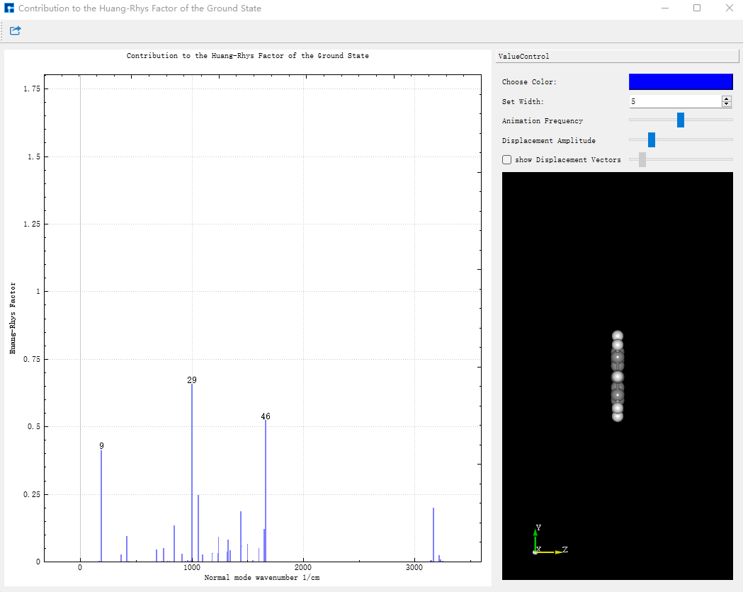
Click Choose Color to change line colors; change the value in Set Width to change line thickness. Clicking on lines in the diagram displays the corresponding vibration mode on the right structure. Vibration speed can be adjusted via Animation Frequency; vibration amplitude can be displayed via Displacement Amplitude.
Next, perform fluorescence spectrum and fluorescence radiative rate calculation for S₁→S₀. This calculation requires the evc.*.dat file from the EVC calculation as input. As mentioned earlier, place evc.cart.dat in the fluorescence spectrum and radiative rate calculation folder. The input file momap.inp is:
do_spec_tvcf_ft   = 1
do_spec_tvcf_spec = 1

&spec_tvcf
  DUSHIN        = .t.
  Temp          = 300 K
  tmax          = 1000 fs
  dt            = 1   fs
  Ead           = 0.07502 au
  EDMA          = 0.9267 debye
  EDME          = 0.6507 debye
  FreqScale     = 0.70
  DSFile        = "evc.cart.dat"
  Emax          = 0.3 au
  dE            = 0.00001 au
  logFile       = "spec.tvcf.log"
  FtFile        = "spec.tvcf.ft.dat"
  FoFile        = "spec.tvcf.fo.dat"
  FoSFile       = "spec.tvcf.spec.dat"
/
Submit the script file momap.slurm. After the job completes, the following files are generated:
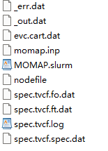
spec.tvcf.ft.dat is the correlation function file, with content like:
[File content unchanged - same as original]
After calculation, first confirm if the correlation function converges. Drag spec.tvcf.ft.dat into Origin, select columns 1 and 2 to plot:
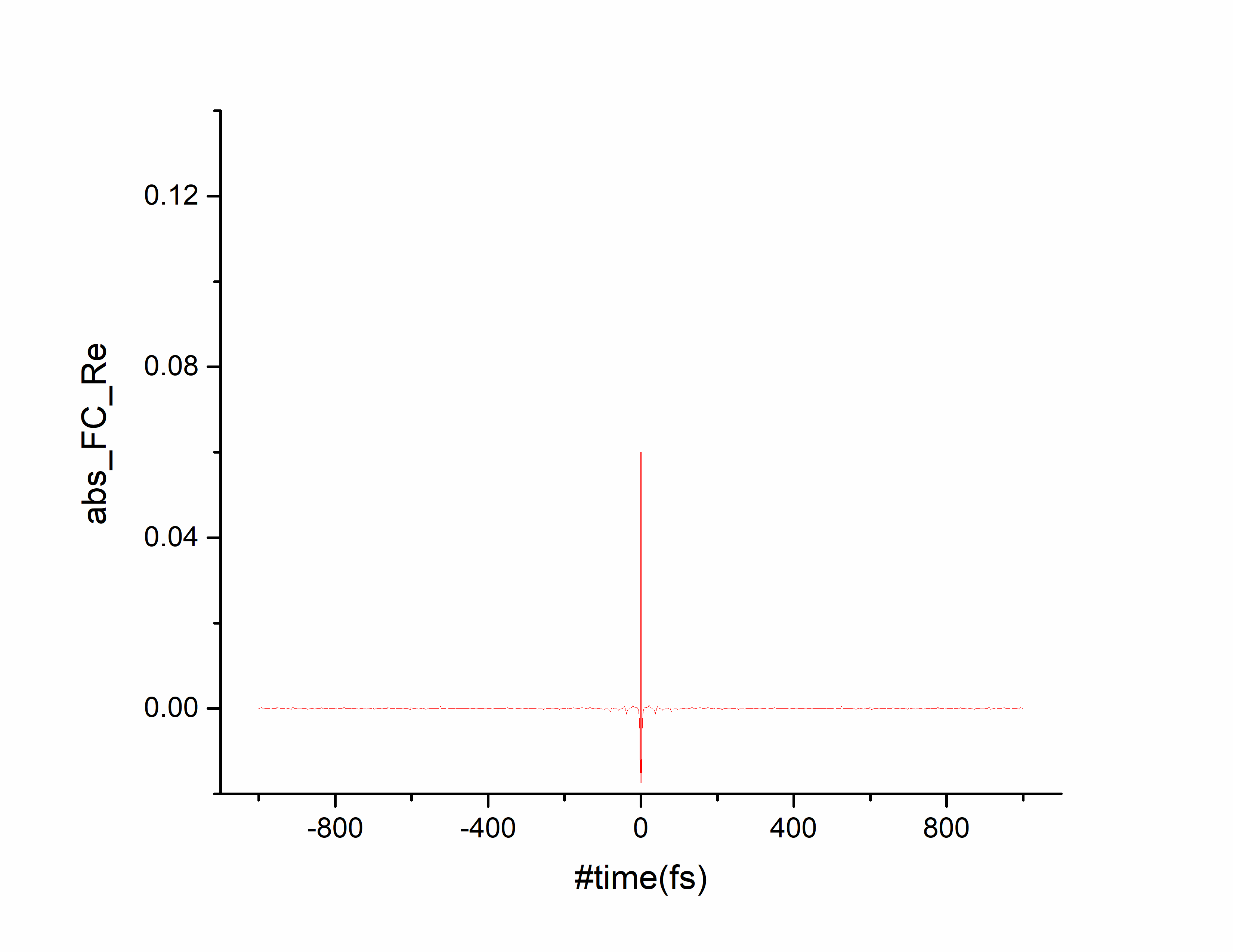
Tending to 0 over time indicates convergence of the absorption spectrum calculation. Select columns 1 and 4 to plot:
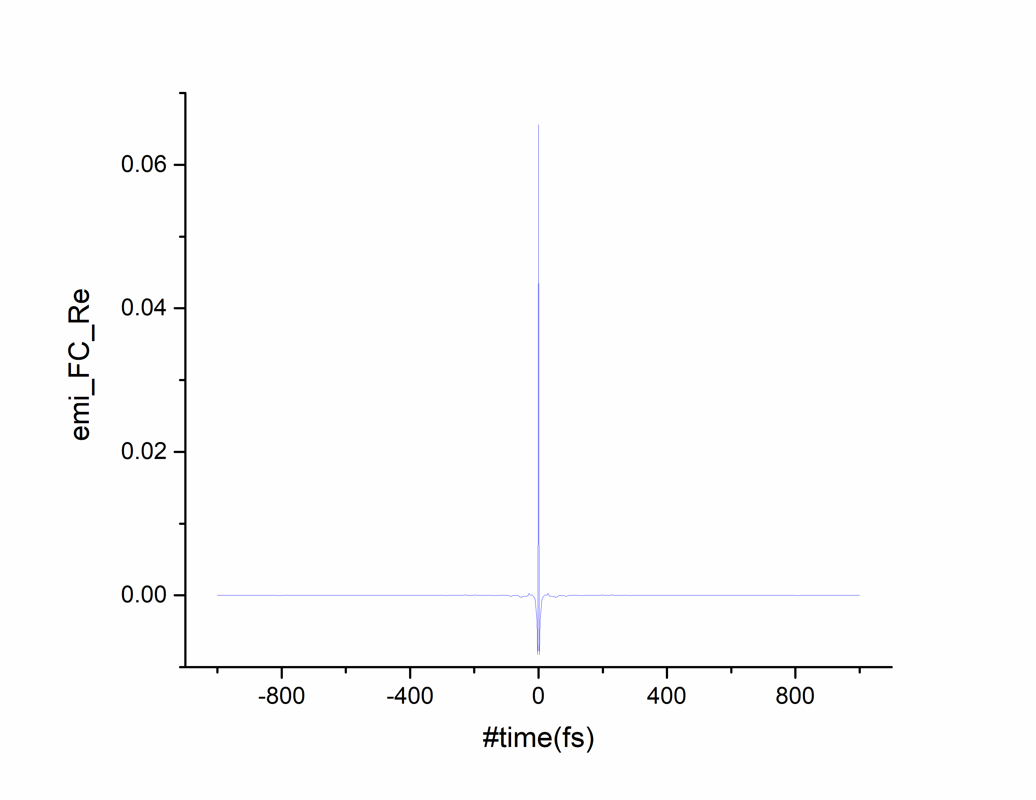
Tending to 0 over time indicates convergence of the emission spectrum calculation.
spec.tvcf.spec.dat is the spectrum file:
[File content unchanged - same as original]
Drag spec.tvcf.spec.dat into Origin, select columns 3 and 5 to plot, obtaining the absorption spectrum:
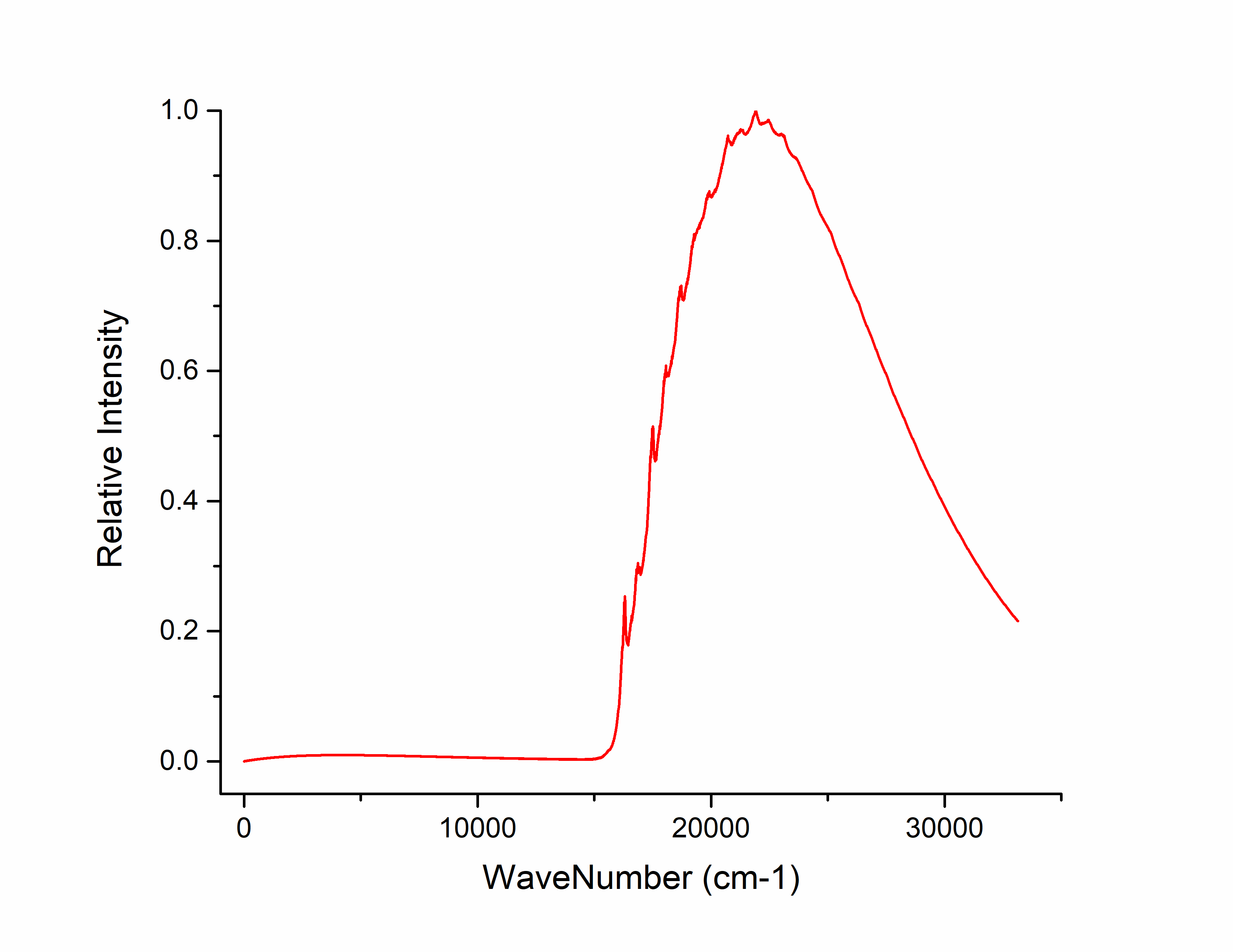
Select columns 3 and 6 to plot, obtaining the emission spectrum:
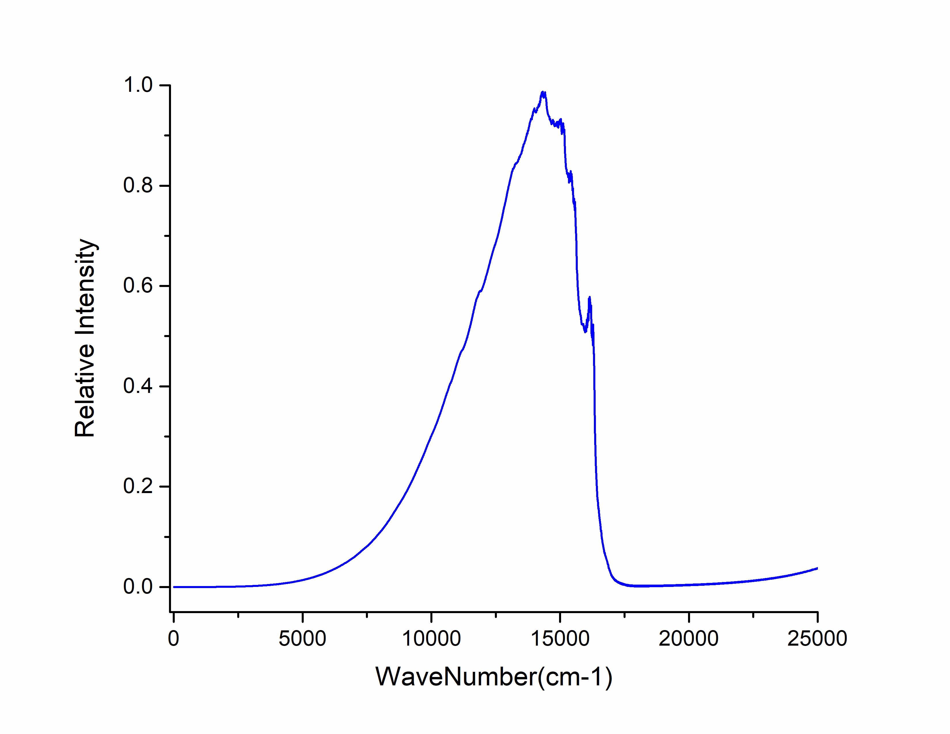
Open spec.tvcf.log, the file outputs the fluorescence radiative rate value at the end:
radiative rate (0): 7.21227543E-12 2.98165371E+05 /s, 3353.84 ns
The fluorescence radiative rate is read from the first and second numbers, with units a.u. and \(s^{-1}\) respectively. The third number is the fluorescence lifetime in ns. Here, azulene’s S₁→S₀ fluorescence radiative rate is 2.98165371E+05 /s, and fluorescence lifetime is 3353.84 ns.
Next, calculate azulene’s internal conversion rate. The first step is EVC vibrational analysis calculation.
The EVC vibrational analysis calculation for internal conversion rate requires the non-adiabatic coupling calculation result file. Rename the non-adiabatic coupling calculation result file to azulene-nacme.out, and place it with azulene-s0.out and azulene-s1.out in the internal conversion rate calculation folder. The input file momap.inp is:
do_evc          = 1

&evc
  ffreq(1)      = "azulene-s0.log"
  ffreq(2)      = "azulene-s1.log"
  fnacme        = "azulene-nacme.log"
  proj_reorg = .t.
/
Submit the script file momap.slurm. After the job completes, the following files are generated:
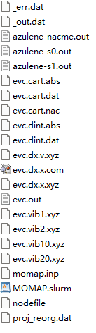
Compared to the previous EVC calculation for fluorescence radiative rate, there is an additional evc.cart.nac file, which will be used together with the evc.cart.dat file for the subsequent internal conversion rate calculation.
The input file for internal conversion rate momap.inp is:
do_ic_tvcf_ft   = 1
do_ic_tvcf_spec = 1

&ic_tvcf
  DUSHIN        = .t.
  Temp          = 300 K
  tmax          = 1000 fs
  dt            = 1   fs
  Ead           = 0.07502 au
  FreqScale     = 0.40
  DSFile        = "evc.cart.dat"
  CoulFile      = "evc.cart.nac"
  Emax          = 0.3 au
  logFile       = "ic.tvcf.log"
  FtFile        = "ic.tvcf.ft.dat"
  FoFile        = "ic.tvcf.fo.dat"
/
After calculation, the following files are generated:
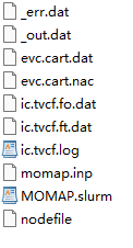
ic.tvcf.ft.dat is the correlation function file, with content like:
[File content unchanged - same as original]
After calculation, first confirm if the correlation function converges. Drag ic.tvcf.ft.dat into Origin, select columns 1 and 2 to plot:
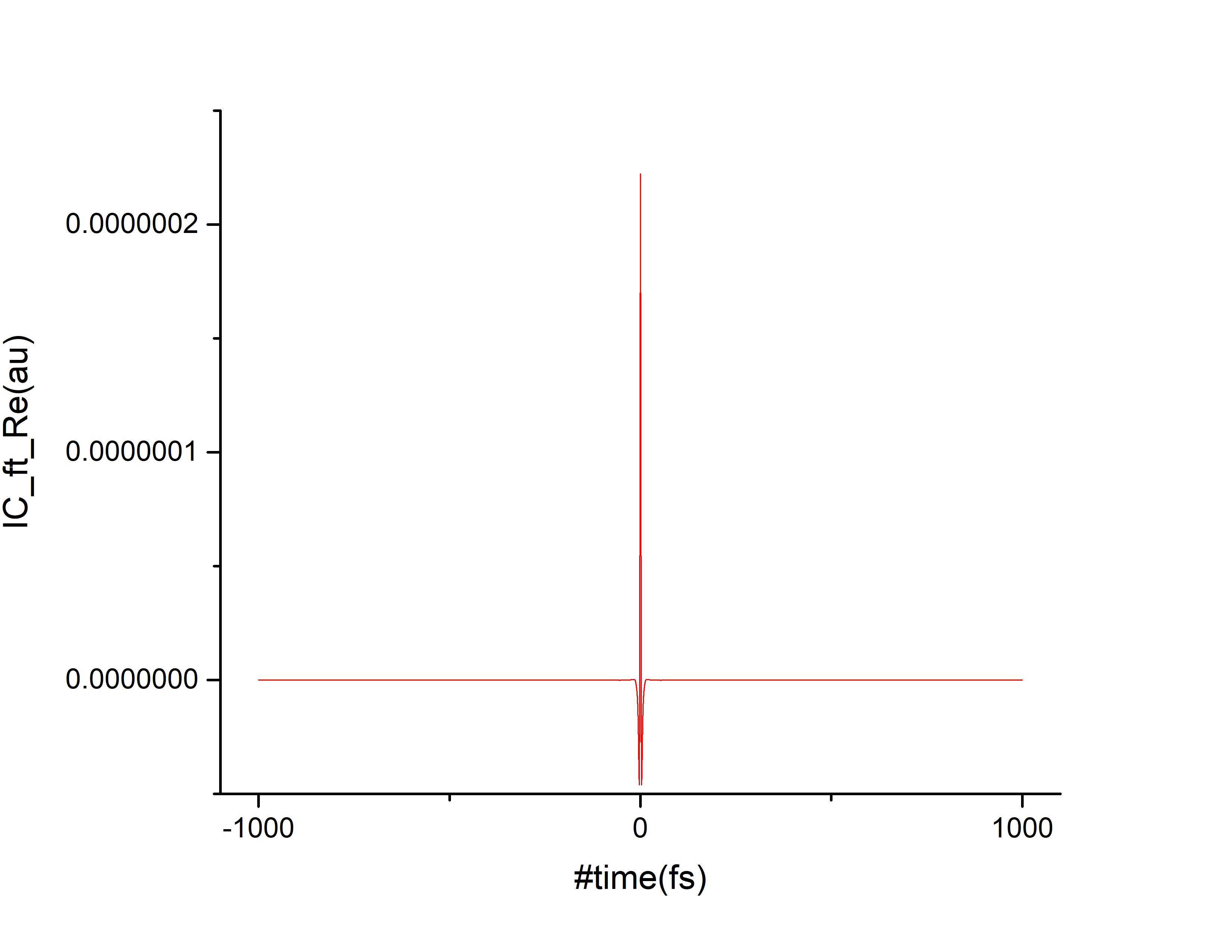
Tending to 0 over time indicates convergence of the correlation function.
ic.tvcf.fo.dat is the spectral function file, with content like:
[File content unchanged - same as original]
To check if it satisfies the energy gap law, drag ic.tvcf.fo.dat into Origin, select columns 3 and 7 to plot:
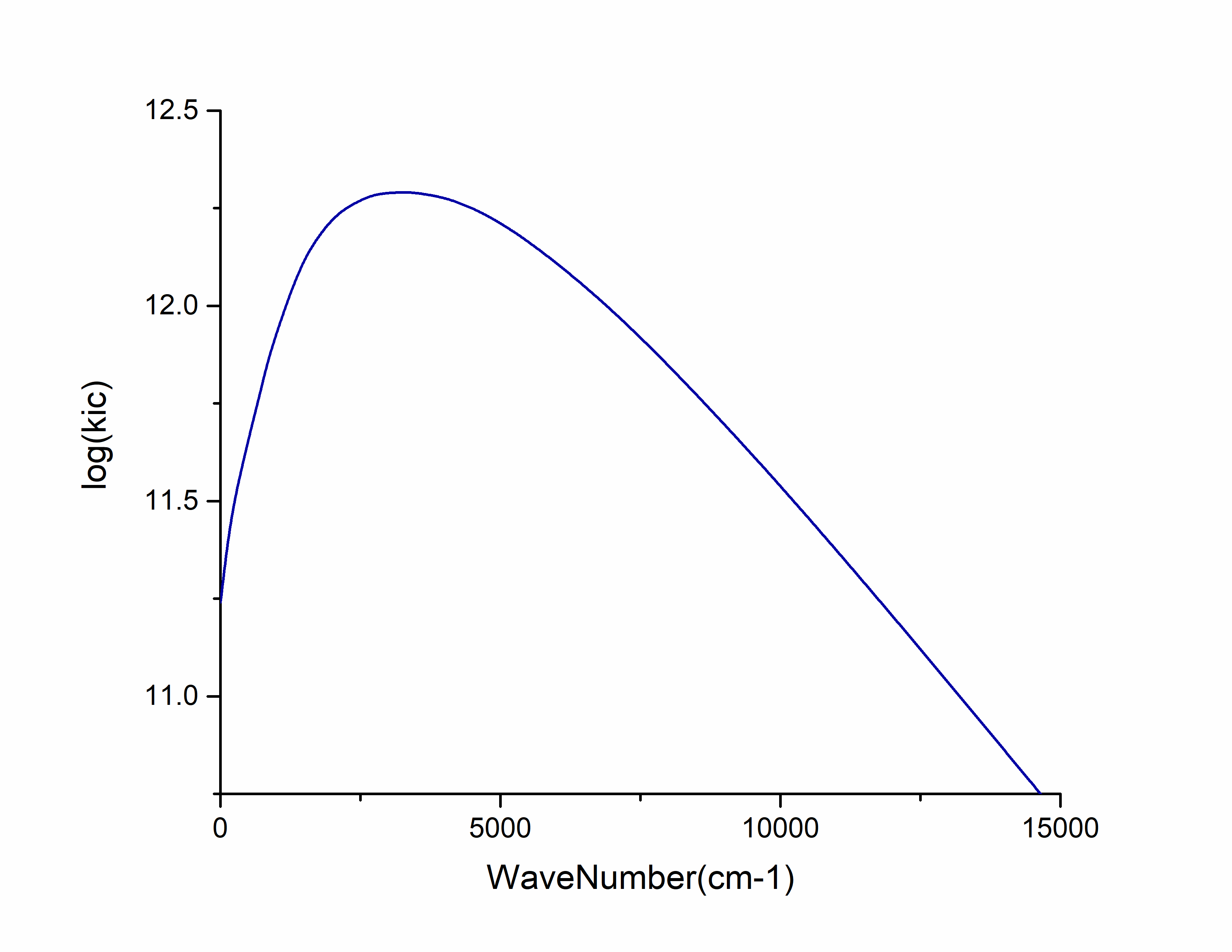
Additionally, columns 1 and 6 in the ic.tvcf.fo.dat file represent the non-radiative rates at different Ead values.
In the ic.tvcf.log file at the end, read the non-radiative rate value of S₁→S₀:
 #1Energy(Hartree)       2Energy(eV) 3WaveNumber(cm-1)   4WaveLength(nm)    5radi-spectrum      6kic(s^{-1})         7log(kic)         8time(ps)
7.50036029E-02    2.04095275E+00    1.64613880E+04    6.07482186E+02    6.54396018E-07    2.70536301E+10    1.04322255E+01       36.96361624
Here, the S₁→S₀ non-radiative rate is 2.70536301E+10 \(s^{-1}\).
Comparing azulene’s fluorescence radiative rate and non-radiative rate: fluorescence radiative rate is 2.98165371E+05 /s, non-radiative rate is 2.70536301E+10 \(s^{-1}\). The non-radiative rate is five orders of magnitude higher than the fluorescence radiative rate, thereby reducing the fluorescence quantum efficiency of azulene’s S₁→S₀ transition and making the S₁→S₀ fluorescence difficult to observe. This results in the anti-Kasha rule fluorescence phenomenon.
Studying Spin-Forbidden Multi-State Reactions with the MSSM Model
In most chemical reaction processes, the system starts from reactants, passes through one or more transition states and intermediates, and finally reaches products—all occurring on the ground-state potential energy surface. However, in some cases, reactants, transition states, intermediates, or products may reside on potential energy surfaces of different spin states. Such reactions are termed spin-forbidden reactions or multi-state reactions, hereafter abbreviated as multi-state reactions. These reactions occur due to spin-orbit coupling and pose theoretical challenges.
Note
Most multi-state reactions involve only two spin states and are sometimes called two-state reactions in the literature.
Spin-conserved chemical reactions may also occur on two (or more) potential energy surfaces of the same spin state, but this is difficult to detect without IRC optimization. Such cases can be handled by conventional theoretical methods and are not classified as multi-state reactions.
Strictly incorporating spin-orbit coupling in chemical reactions requires two-component or four-component relativistic methods (especially two/four-component relativistic density functional theory, which has analytic gradients implemented in some quantum chemistry programs). However, due to practical difficulties, these methods are rarely applied. If spin-orbit coupling is weak, the minimum energy crossing point (MECP) method can approximate the lowest energy intersection between spin-state potential energy surfaces (see MECP). Although widely used, MECP has limitations: (1) If MECP corresponds to a new transition state, its vibrational frequencies and thermochemical properties cannot be obtained since MECP is not a true stationary point; (2) MECP cannot handle simultaneous crossings of more than two spin states or crossings within small regions; (3) For 3d elements, MECP positions and energies can deviate significantly from two-component relativistic results [94]; (4) MECP is unsuitable for actinide systems; its applicability to unsaturated-bonded 5d systems is questionable.
In 2018, Truhlar et al. proposed the two-state spin-mixing (TSSM) model to simulate spin-orbit coupling between two spin states during chemical reactions [83]. Recently, we generalized it to the multi-state spin-mixing (MSSM) model, applicable to multiple spin states. MSSM avoids the first three drawbacks of MECP and is suitable for elements up to 5d [95]. Tests on 5d compound reactions show that MSSM-DFT reaction energies and transition state barriers differ by less than 3 kcal/mol from two-component DFT results (for unsaturated-bonded 5d compounds, two/four-component single-point energy corrections are needed).
As an example, we use the MSSM model to repeat Truhlar’s TSSM study of the dehydrogenation reaction in a tungsten complex: \(W(CH_3)(n-C_3H_7)(OH)_2 \rightarrow WH(CH_3)(=CHC_2H_5)(OH)_2\) [83]. In the literature, this system approximates a heterogeneous tungsten catalyst for atomic layer deposition, where the support skeleton is replaced by two OH groups. The reaction schematic is shown below: blue lines indicate the singlet reaction path, red lines the triplet path, black lines the lowest energy path after spin mixing, and yellow lines the singlet contribution to the lowest mixed state. During the reaction, tungsten’s oxidation state changes from +4 to +6. In the reactant, tungsten is partially coordinated, making the triplet state lowest in energy (spin-mixed ground state dominated by triplet). In the product, tungsten is fully coordinated, making the closed-shell singlet lowest (spin-mixed ground state dominated by singlet). The triplet-singlet crossing point and the transition state of the spin-mixed ground state are separated (though energetically close), with the singlet contributing ~90% at the transition state—a key difference from MECP where spins mix 1:1.
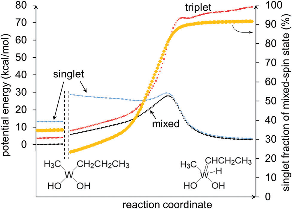
Generally, before MSSM calculations, conventional scalar methods should optimize reactant, product, transition state, and intermediate structures for all possible spin states to identify critical spin states and initial structures for MSSM optimization. Since this reaction is well-studied [83], we skip this step and directly optimize reactant, product, and transition state structures on the spin-mixed ground-state potential energy surface using MSSM, then compute vibrational frequencies. Initial coordinates are taken from the literature. Basis sets: def2-TZVP for W, 6-31G* for other atoms. The empirical SOC parameter is 302 meV (2436 \(\rm cm^{-1}\)) from the literature. We replace M06L with B3LYP for better numerical stability. Results are compared with TSSM [83] and two-component relativistic data [95]:
More applications can be found in the Takayanagi group’s series of papers. They used TSSM to study numerous two-state reactions involving 3d/4d elements (see [84] and its citations).
BDF Calculation Input
Input for optimizing the spin-mixed ground state reactant is shown below. For command explanations, see comments in the ZnS spin-mixed state example.
$compass
title
   W system: reactant
basis-block
 6-31G*
 W=def2-tzvp
end basis
# geom from PCCP 2018, 20, 4129
geometry
C  -2.50599000   0.80875000   0.27831700
H  -2.42978000   0.87169600   1.37614800
H  -3.29329400   1.52978300   0.00369300
C  -1.17932200   1.22962500  -0.35262900
H  -1.30089800   1.27432600  -1.45149600
W   0.49596700  -0.04848100   0.05050100
H  -0.94880200   2.26591700  -0.04284700
C  -2.96148400  -0.58790000  -0.11445500
H  -2.28153800  -1.36238600   0.26893400
H  -3.96244500  -0.81403100   0.27115200
H  -2.98974600  -0.70153100  -1.20640700
O   1.64397700   1.44403300  -0.35823300
H   1.22595200   2.31740600  -0.43846900
O   0.49410200  -0.94895200   1.73966100
H  -0.19914300  -0.83307900   2.40480100
C   0.26970600  -1.43014300  -1.54486300
H  -0.59187900  -2.09433400  -1.38019500
H   0.07131900  -0.88842400  -2.48170400
H   1.15657400  -2.06035000  -1.71035900
end geometry
nosymm
$end

$bdfopt
multistate
 2soc  2436
solver
 1
hess
 final
$end

$xuanyuan
$end

%cp $BDF_WORKDIR/$BDFTASK.scforb.1   $BDF_WORKDIR/$BDFTASK.scforb    2>/dev/null || :
$scf
rks
dft
 b3lyp
grid
 fine
$end
%cp $BDF_WORKDIR/$BDFTASK.scforb     $BDF_WORKDIR/$BDFTASK.scforb.1

$resp
geom
$end
%cp $BDF_WORKDIR/$BDFTASK.egrad1     $BDF_WORKDIR/$BDFTASK.egrad.1   2>/dev/null || :
%cp $BDF_WORKDIR/$BDFTASK.hess       $BDF_WORKDIR/$BDFTASK.hess.1    2>/dev/null || :

%cp $BDF_WORKDIR/$BDFTASK.scforb.2   $BDF_WORKDIR/$BDFTASK.scforb    2>/dev/null || :
$scf
uks
dft
 b3lyp
spinmulti
 3
grid
 fine
$end
%cp $BDF_WORKDIR/$BDFTASK.scforb     $BDF_WORKDIR/$BDFTASK.scforb.2

$resp
geom
$end
%cp $BDF_WORKDIR/$BDFTASK.egrad1     $BDF_WORKDIR/$BDFTASK.egrad.2   2>/dev/null || :
%cp $BDF_WORKDIR/$BDFTASK.hess       $BDF_WORKDIR/$BDFTASK.hess.2    2>/dev/null || :
Input for optimizing the spin-mixed ground state product is similar. Only the compass module is shown below; other sections match the reactant input.
$compass
title
   W system: product
basis-block
 6-31G*
 W=def2-tzvp
end basis
# geom from PCCP 2018, 20, 4129
geometry
W  -0.42387000  -0.03021600  0.04243900
O  -0.54695900  -1.59597800 -1.06031400
H  -1.38476400  -2.05907900 -0.89227700
O  -2.07683400  -0.36779800  1.01946300
H  -2.09920000  -0.45365300  1.97932500
C  -1.19429700   1.74966400 -0.81144000
H  -1.16507500   2.46066600  0.03099700
H  -0.64596000   2.20075800 -1.64296300
H  -2.24817300   1.61217900 -1.08859500
H   0.10061200   0.01381000  1.68243000
C   1.39659000   0.37442700 -0.02642700
H   1.22850000   0.24599300 -1.14781000
C   2.78803600   0.62890000  0.40356700
H   2.79144700   0.71717400  1.49877400
H   3.12713400   1.60782200  0.02677600
C   3.77244700  -0.45270200 -0.03426000
H   4.78897300  -0.22737400  0.30879300
H   3.48486900  -1.42988500  0.36906600
H   3.80168700  -0.54392400 -1.12680400
end geometry
nosymm
$end
For the spin-mixed ground state transition state, modify only the compass and bdfopt modules in the reactant input:
$compass
title
   W system: TS
basis-block
 6-31G*
 W=def2-tzvp
end basis
# geom from PCCP 2018, 20, 4129
geometry
C   2.75476500  -0.49692100  0.66265200
H   2.66846800  -0.03811600  1.65776400
H   3.19563100  -1.49505600  0.81976100
C   1.39220000  -0.59199800  0.03929900
H   1.40125200  -1.14322200 -0.93707500
W  -0.48542700  -0.04574900 -0.00978200
H   0.62772500  -0.92650400  1.07995600
C   3.68608400   0.33536600 -0.20966500
H   3.29355400   1.35035000 -0.34119700
H   4.68482600   0.40829800  0.23538400
H   3.79640600  -0.10658300 -1.20747300
O  -1.41339700  -1.47110300 -0.89277200
H  -1.32731100  -2.36616000 -0.52320400
O  -1.79388100   0.67727500  1.22320500
H  -1.75031500   0.44148600  2.15765700
C  -0.22357400   1.89123400 -0.83239900
H   0.11804400   2.54791300 -0.01489800
H   0.44852800   2.01363400 -1.68618700
H  -1.23385200   2.22393900 -1.11944000
end geometry
nosymm
$end

$bdfopt
multistate
 2soc  2436
solver
 1
hess
 init+final
iopt
 10
$end