Structural optimization and frequency calculation
The purpose of structural optimization is to find the minimum point of the potential energy surface of the system. Which minimum point can be found depends on the initial structure provided in the input file, and the closer you are to which minimum point, the easier it is to converge to which minimum point.
Structural optimization is mathematically equivalent to finding the extrema of multivariate functions:
Common algorithms for structural optimization are as follows:
Steepest descent: The fastest descent method is to search for lines along the direction of the negative gradient, and the optimization efficiency of the fastest descent method is very high for structures far away from the minimum point, but the convergence is slow and easy to oscillate when it is close to the minimum point.
Conjugate gradient: The conjugate gradient method is an improvement of the fastest descent method, and the optimization direction of each step is combined with the optimization direction of the previous step, which can alleviate the oscillation problem to a certain extent.
Newton method: The idea of Newton’s method is to expand a function in a Taylor series relative to its current position. Newton’s method converges quickly, and for quadratic functions, it can reach a minimum point in one step. However, Newton’s method requires solving Hessian matrices, which is very expensive to calculate, and quasi-Newton’s method is used in general geometric optimization.
Quasi-Newton method: The quasi-Newton method constructs the Hessian matrix by approximating the Hessian matrix, and the Hessian matrix of the current step is obtained based on the force of the current step and the Hessian matrix of the previous step. There are many specific methods, the most commonly used is the BFGS method, in addition to DFP, MS, PSB, etc. Since the Hessian of the quasi-Newtonian method is constructed approximately, the accuracy of each step of optimization is lower than that of the Newtonian method, and the number of steps required to achieve convergence is more than that of the Newtonian method. However, due to the significant reduction in the time required for each step, the total optimization time is significantly reduced.
The structural optimization of BDF is realized by the BDFOPT module, which supports the optimization of the minimum point structure and transition state structure based on the Newton method and the quasi-Newton method, and supports the optimization of restrictive structure. The following is an example of the input file format of the BDFOPT module and the interpretation of the output file.
Ground-state structure optimization: Structural optimization of monochloromethane ( :math:’ce{CH3Cl}’ at B3LYP/def2-SV(P) levels
$compass
title
   CH3Cl geomopt
basis
   def2-SV(P)
geometry
 C                  2.67184328    0.03549756   -3.40353093
 H 2.05038141 -0.21545378 -2.56943947
 H 2.80438882 1.09651909 -3.44309081
 H 3.62454948 -0.43911916 -3.29403269
 Cl 1.90897396 -0.51627638 -4.89053325
end geometry
$end

$bdfopt
solver
 1
$end

$xuanyuan
$end

$scf
rks
dft
 b3lyp
$end

$resp
Geom
$end
The RESP module is responsible for calculating the DFT gradient. Unlike most other tasks, in the structural optimization task, the program does not call the modules sequentially, singlely, and linearly, but calls them multiple times. The specific order of invocation is as follows:
Run COMPASS to read molecular structure and other information;
Run BDFOPT to initialize the intermediate amount required for structural optimization;
BDFOPT starts an independent BDF process to calculate the energy and gradient under the current structure, which only executes the COMPASS, XUANYUAN, SCF, and RESP modules, and skips BDFOPT. In other words, most of the time you will find that there are two BDF processes running independently of each other, one of which is the BDFOPT process and is waiting, while the other process is performing energy and gradient calculations. In order to avoid cluttering the output file, the output of the latter process will be automatically redirected to a file with the suffix “.out.tmp”, which is separate from the output of the BDFOPT module (which is usually redirected to the “.out” file by the user);
At the end of the latter process, BDFOPT summarizes the energy and gradient information of the current structure, and adjusts the molecular structure accordingly to reduce the energy of the system.
BDFOPT determines whether the structure converges according to the gradient of the current structure and the size of the current geometry step. If not, skip to step 3.
Therefore, the .out file only contains the output of the COMPASS and BDFOPT modules, which can be used to monitor the progress of structural optimization, but does not contain information such as SCF iteration and distribution analysis, which needs to be viewed in the .out.tmp file.
Taking the above :math:’ce{CH3Cl} structure optimization task as an example, you can see the output of the BDFOPT module in the .out file:
   Geometry Optimization step :    1

  Single Point SCF for geometry optimization, also get force.


 ### [bdf_single_point] ### nstate= 1
 Allow rotation to standard orientation.

 BDFOPT run - details of gradient calculations will be written
 into .out.tmp file.

...

### JOB TYPE = SCF ###
E_tot= -499.84154693
Converge= YES

### JOB TYPE = RESP_GSGRAD ###
Energy= -499.841546925072
     1        0.0016714972        0.0041574983       -0.0000013445
     2       -0.0002556962       -0.0006880567        0.0000402277
     3       -0.0002218807       -0.0006861734       -0.0000225761
     4       -0.0003229876       -0.0006350885       -0.0000059774
     5       -0.0008670369       -0.0021403962       -0.0000084046
It can be seen that BDFOPT calls the BDF program itself to calculate the SCF energy and gradient of the molecule under the initial guess structure. The detailed output of the SCF and gradient calculations is in the .out.tmp file, while the .out file only extracts information such as energy values, gradient values, and whether the SCF converges. The unit of energy is Hartree, and the unit of gradient is Hartree/Bohr.
‘’solver’’ = 1 indicates that the structure is optimized in redundant internal coordinates using BDF’s own optimizer. In order to generate the next molecular structure, the redundant internal coordinates of the molecule must first be generated. Therefore, in the first step of structural optimization, the output file will also give the definition of the coordinates in each redundancy (i.e., the atomic numbers involved in the formation of the corresponding bonds, bond angles, and dihedral angles). and their values (the unit of bond length is angstroms, and the unit of bond angle, dihedral angle is degrees):
|******************************************************************************|
       Redundant internal coordinates on Angstrom/Degree

  Name         Definition         Value     Constraint
  R1 1 2 1.0700 No
  R2 1 3 1.0700 No
  R3 1 4 1.0700 No
  R4 1 5 1.7600 No
  A1 2 1 3 109.47 No
  A2 2 1 4 109.47 No
  A3 2 1 5 109.47 No
  A4 3 1 4 109.47 No
  A5 3 1 5 109.47 No
  A6 4 1 5 109.47 No
  D1 4 1 3 2 -120.00 No
  D2 5 1 3 2 120.00 No
  D3 2 1 4 3 -120.00 No
  D4 3 1 4 2 120.00 No
  D5 5 1 4 2 -120.00 No
  D6 5 1 4 3 120.00 No
  D7 2 1 5 3 120.00 No
  D8 2 1 5 4 -120.00 No
  D9 3 1 5 2 -120.00 No
  D10 3 1 5 4 120.00 No
  D11 4 1 5 2 120.00 No
  D12 4 1 5 3 -120.00 No

|******************************************************************************|
After the molecular structure update is completed, the program calculates the gradient and the size of the geometric step to determine whether the structure optimization is convergent:
                   Force-RMS    Force-Max     Step-RMS     Step-Max
Conv. tolerance :  0.2000E-03   0.3000E-03   0.8000E-03   0.1200E-02
Current values  :  0.8833E-02   0.2235E-01   0.2445E-01   0.5934E-01
Geom. converge  :     No           No           No           No
Only when the current values of Force-RMS, Force-Max, Step-RMS, and Step-Max are all less than the corresponding convergence limit (i.e., Geom. converge’’ column is Yes), the program considers the structure to be optimized and converged. For this example, the structure optimization converges in step 5, and the output information not only contains the values of each convergence criterion, but also explicitly informs the user that the geometric optimization has converged, and prints the converged molecular structures in the form of Cartesian coordinates and internal coordinates, respectively:
    Good Job, Geometry Optimization converged in     5 iterations!

   Molecular Cartesian Coordinates (X,Y,Z) in Angstrom :
      C          -0.93557703       0.15971089       0.58828595
      H -1.71170348 -0.52644336 0.21665897
      H -1.26240747 1.20299703 0.46170050
      H -0.72835075 -0.04452039 1.64971607
      Cl 0.56770184 -0.09691413 -0.35697029

                       Force-RMS    Force-Max     Step-RMS     Step-Max
    Conv. tolerance :  0.2000E-03   0.3000E-03   0.8000E-03   0.1200E-02
    Current values  :  0.1736E-05   0.4355E-05   0.3555E-04   0.6607E-04
    Geom. converge  :     Yes          Yes          Yes          Yes


  Print Redundant internal coordinates of the converged geometry

|******************************************************************************|
       Redundant internal coordinates on Angstrom/Degree

  Name         Definition         Value     Constraint
  R1 1 2 1.1006 No
  R2 1 3 1.1006 No
  R3 1 4 1.1006 No
  R4 1 5 1.7942 No
  A1 2 1 3 110.04 No
  A2 2 1 4 110.04 No
  A3 2 1 5 108.89 No
  A4 3 1 4 110.04 No
  A5 3 1 5 108.89 No
  A6 4 1 5 108.89 No
  D1 4 1 3 2 -121.43 No
  D2 5 1 3 2 119.28 No
  D3 2 1 4 3 -121.43 No
  D4 3 1 4 2 121.43 No
  D5 5 1 4 2 -119.28 No
  D6 5 1 4 3 119.29 No
  D7 2 1 5 3 120.00 No
  D8 2 1 5 4 -120.00 No
  D9 3 1 5 2 -120.00 No
  D10 3 1 5 4 120.00 No
  D11 4 1 5 2 120.00 No
  D12 4 1 5 3 -120.00 No

|******************************************************************************|
Note that the convergence limits of the RMS force and RMS step can be set by the keywords ‘’tolgrad’’ and ‘’tolstep’’’ respectively, and the program automatically adjusts the convergence limits of the maximum force and the maximum step size according to the set values. When using the DL-FIND library (see below), it is also possible to specify the energy convergence limit using tolene. However, it is generally not recommended that users adjust the convergence limit on their own.
At the same time, the program will also generate a file with the suffix “.optgeom”, which contains the Cartesian coordinates of the optimized molecular structure (or the Cartesian coordinates of the current structure in the standard orientation in the case of a normal single-point calculation), but in Bohr instead of Angstrom:
GEOM
        C             -0.7303234729        -2.0107211546        -0.0000057534
        H -0.5801408002 -2.7816264533 1.9257943885
        H 0.4173171420 -3.1440530286 -1.3130342173
        H -2.7178161476 -2.0052051760 -0.6126883555
        Cl 0.4272106261 1.1761889168 -0.0000021938
The .optgeom file can be converted to xyz format using the tool optgeom2xyz.py under $BDFHOME/sbin/, so that the optimized molecular structure can be viewed in any visualization software that supports the xyz format. For example, if the file to be converted is named filename.optgeom, execute the following command line (note that you must first set the environment variable $BDFHOME, or manually replace $BDFHOME with the path of the BDF folder in the following command)
$BDFHOME/sbin/optgeom2xyz.py filename
The filename.xyz will be available in the current directory.
Note
Although the coordinates in the .xyz file obtained from the above steps are in Angstrom, the values may not be the same as the coordinates in the .out file, which is normal because the numerator orientation and coordinate origin of the two files are different. In the same way, the coordinates in the .optgeom file and the coordinates in the .out file are not simple unit conversions, but may differ from one translation and one rotation.
Finally, it is pointed out that when the bond angle in the molecule is close to or equal to 180 degrees, the optimization algorithm based on redundant internal coordinates often has the problem of numerical instability, which makes the optimization unable to continue. Therefore, when generating redundant internal coordinates, the program will try to avoid selecting a key angle close to or equal to 180 degrees. However, even so, there is still a possibility that the bond angle that was much less than 180 degrees will be close to 180 degrees during the optimization process, resulting in the problem of numerical instability, at this time, the program will automatically reconstruct the redundant internal coordinates and automatically restart the optimization, and output the following information:
 Something wrong in getting dihedral!
 This is probably because one or more angles have become linear.


--- Restarting optimizer ... (10 attempt(s) remaining) ---
As can be seen from the output information, the program allows the optimizer to restart a total of 10 times. Under normal circumstances, the structure can be successfully optimized by restarting the optimizer only 1~2 times, but in rare cases, after the 10 restart opportunities are exhausted, the key angle will still be close to 180 degrees, and the program will exit with an error:
bdfopt_bdf: fatal: the maximum number of restarts has been reached
Please check if your geometry makes sense!
In this case, the user should check whether the current coordinates in the .optgeom file are reasonable, if so, you can use the DL-Find optimizer to optimize in Cartesian coordinates, see Geometry Optimization Non-Convergent Solution <geomoptnotconverged> for details.
Frequency calculation::math:’ce{CH3Cl}’ Calculation of resonant frequency and thermochemical quantity in equilibrium structure
Once the structure is optimized and converged, the frequency analysis can be performed. Prepare the following input files:
$compass
title
 CH3Cl freq
basis
 def2-SV(P)
geometry
 C          -0.93557703       0.15971089       0.58828595
 H -1.71170348 -0.52644336 0.21665897
 H -1.26240747 1.20299703 0.46170050
 H -0.72835075 -0.04452039 1.64971607
 Cl 0.56770184 -0.09691413 -0.35697029
end geometry
$end

$bdfopt
hess
 only
$end

$xuanyuan
$end

$scf
rks
dft
 b3lyp
$end

$resp
Geom
$end
The molecular structure is the convergent structure obtained by the above structure optimization tasks. Note that we have added ‘’hess only’’ to the BDFOPT module, where ‘hess’’ stands for computational (numeric) Hessian, and the meaning of ‘’only’’ will be explained in more detail in a later section. The program perturbates each atom in the molecule in the positive x-axis, negative x-axis, y-positive direction, y-negative direction, z-axis positive direction, and z-axis negative direction, and calculates the gradient under the perturbation structure, such as:
 Displacing atom    1 (+x)...

 ### [bdf_single_point] ### nstate= 1
 Do not allow rotation to standard orientation.

 BDFOPT run - details of gradient calculations will be written
 into .out.tmp file.

...

### JOB TYPE = SCF ###
E_tot= -499.84157717
Converge= YES

### JOB TYPE = RESP_GSGRAD ###
Energy= -499.841577166026
     1        0.0005433780       -0.0000683370       -0.0000066851
     2       -0.0000516384        0.0000136326       -0.0000206081
     3       -0.0001360377        0.0000872513        0.0000990006
     4       -0.0003058645        0.0000115926       -0.0000775624
     5       -0.0000498284       -0.0000354732        0.0000023346
Note
Since the perturbation structure will break the point group symmetry of the molecule, even if there is point group symmetry in the user’s input molecule, the calculation will automatically be changed to the C(1) group. If you want to specify the number of orbits occupied by each irreducible representation, or calculate the numerical frequency of an excited state under a specific irreducible representation, you must first do a separate single-point calculation to maintain the symmetry of the point group, manually specify which orbit or excited state you want to occupy or which orbit or excited state you want to calculate corresponds to the C(1) group according to the results of the single-point calculation, and then write the numerical frequency calculation input file under the C(1) group according to the designation results.
If the number of atoms in the system is N, a total of 6N gradients need to be calculated. However, in fact, the program will also calculate the gradient of the undisturbed structure in passing, so that the user can check whether the aforementioned structural optimization has indeed converged, so the program actually calculates a total of 6N+1 gradients. Finally, the program uses the finite difference method to obtain the Hessian of the system:
|--------------------------------------------------------------------------------|
          Molecular Hessian - Numerical Hessian (BDFOPT)

                      1              2              3              4              5              6
       1   0.5443095266  -0.0744293569  -0.0000240515  -0.0527420800   0.0127361607  -0.0209022664
       2  -0.0744293569   0.3693301504  -0.0000259750   0.0124150102  -0.0755387479   0.0935518380
       3  -0.0000240515  -0.0000259750   0.5717632089  -0.0213157291   0.0924260912  -0.2929392390
       4  -0.0527420800   0.0124150102  -0.0213157291   0.0479752418  -0.0069459473   0.0239610358
       5   0.0127361607  -0.0755387479   0.0924260912  -0.0069459473   0.0867377886  -0.0978524147
       6  -0.0209022664   0.0935518380  -0.2929392390   0.0239610358  -0.0978524147   0.3068416997
       7  -0.1367366097   0.0869338594   0.0987840786   0.0031968314  -0.0034098009  -0.0016497426
       8   0.0869913627  -0.1185605401  -0.0945336434  -0.0070787068   0.0099076105   0.0045621064
       9   0.0986508197  -0.0953400774  -0.1659434327   0.0163191407  -0.0140134399  -0.0166739137
      10  -0.3054590932   0.0111756577  -0.0774713107   0.0016297078   0.0019657599  -0.0021771884
      11   0.0112823039  -0.0407134661   0.0021058508   0.0106623780   0.0018506067   0.0005120364
      12  -0.0775840113   0.0018141942  -0.0759448618  -0.0275602878   0.0006820252  -0.0059830018
      13  -0.0486857506  -0.0362556088   0.0000641125  -0.0000787206  -0.0045253276   0.0011289985
      14  -0.0360823429  -0.1334063062   0.0000148321  -0.0091074064  -0.0228930763  -0.0010993076
      15   0.0001686252   0.0004961854  -0.0352553706   0.0084860406   0.0189117305   0.0079690194

                      7              8              9             10             11             12
       1  -0.1367366097   0.0869913627   0.0986508197  -0.3054590932   0.0112823039  -0.0775840113
       2   0.0869338594  -0.1185605401  -0.0953400774   0.0111756577  -0.0407134661   0.0018141942
       3   0.0987840786  -0.0945336434  -0.1659434327  -0.0774713107   0.0021058508  -0.0759448618
       4   0.0031968314  -0.0070787068   0.0163191407   0.0016297078   0.0106623780  -0.0275602878
       5  -0.0034098009   0.0099076105  -0.0140134399   0.0019657599   0.0018506067   0.0006820252
       6  -0.0016497426   0.0045621064  -0.0166739137  -0.0021771884   0.0005120364  -0.0059830018
       7   0.1402213115  -0.0861503922  -0.1081442631  -0.0130805143   0.0143574755   0.0192323598
       8  -0.0861503922   0.1322736798   0.1009922720   0.0016534140   0.0024111759   0.0011733340
       9  -0.1081442631   0.1009922720   0.1688786678  -0.0038440081   0.0072277457   0.0091535975
      10  -0.0130805143   0.0016534140  -0.0038440081   0.3186765202  -0.0079165663   0.0838593213
      11   0.0143574755   0.0024111759   0.0072277457  -0.0079165663   0.0509206668  -0.0029665370
      12   0.0192323598   0.0011733340   0.0091535975   0.0838593213  -0.0029665370   0.0707430980
      13   0.0064620333   0.0044161973  -0.0031236007  -0.0026369496  -0.0283860480   0.0017966445
      14  -0.0119743475  -0.0258901434   0.0013817613  -0.0066143965  -0.0145372292  -0.0006143935
      15  -0.0078330845  -0.0126024853   0.0040383425  -0.0008566397  -0.0068931757   0.0018028482

                     13             14             15
       1  -0.0486857506  -0.0360823429   0.0001686252
       2  -0.0362556088  -0.1334063062   0.0004961854
       3   0.0000641125   0.0000148321  -0.0352553706
       4  -0.0000787206  -0.0091074064   0.0084860406
       5  -0.0045253276  -0.0228930763   0.0189117305
       6   0.0011289985  -0.0010993076   0.0079690194
       7   0.0064620333  -0.0119743475  -0.0078330845
       8   0.0044161973  -0.0258901434  -0.0126024853
       9  -0.0031236007   0.0013817613   0.0040383425
      10  -0.0026369496  -0.0066143965  -0.0008566397
      11  -0.0283860480  -0.0145372292  -0.0068931757
      12   0.0017966445  -0.0006143935   0.0018028482
      13   0.0450796910   0.0642866688   0.0000350066
      14   0.0642866688   0.1954779468   0.0000894464
      15   0.0000350066   0.0000894464   0.0213253497

|--------------------------------------------------------------------------------|
Rows 3N+1 (3N+2, 3N+3) correspond to the x(y, z) coordinates of the Nth atom, and columns 3N+1 (3N+2, 3N+3) do the same.
Next, BDF invokes the UniMoVib program to calculate the frequency and thermodynamic quantities. The first is the irreducible representation to which the vibration belongs, the vibration frequency, the reduced mass, the force constant, and the results of the normal mode:
************************************
***  Properties of Normal Modes  ***
************************************

Results of vibrations:
Normal frequencies (cm^-1), reduced masses (AMU), force constants (mDyn/A)

                                                  1                                 2                                 3
         Irreps A1 E E
    Frequencies                            733.9170                         1020.5018                         1021.2363
 Reduced masses                              7.2079                            1.1701                            1.1699
Force constants                              2.2875                            0.7179                            0.7189
       Atom ZA X Y Z X Y Z X Y Z
          1   6        -0.21108  -0.57499  -0.00106      -0.04882   0.01679   0.10300       0.09664  -0.03546   0.05161
          2   1        -0.13918  -0.40351   0.04884      -0.06700  -0.59986  -0.13376      -0.37214  -0.36766  -0.03443
          3   1        -0.11370  -0.42014  -0.03047       0.26496   0.65294  -0.15254      -0.28591  -0.18743  -0.15504
          4   1        -0.19549  -0.38777  -0.01079       0.05490  -0.14087  -0.24770       0.15594   0.73490  -0.07808
          5  17         0.08533   0.23216   0.00014       0.00947  -0.00323  -0.01995      -0.01869   0.00699  -0.01000
The vibration modes are arranged in order of vibration frequency from smallest to largest, and the virtual frequency is ranked in front of all the real frequencies, so the number of virtual frequencies can be known by simply checking the first few frequencies. Next, print the results of the thermochemical analysis:
*********************************************
***   Thermal Contributions to Energies   ***
*********************************************

Molecular mass            :        49.987388    AMU
Electronic total energy   :      -499.841576    Hartree
Scaling factor of Freq.   :         1.000000
Tolerance of scaling      :         0.000000    cm^-1
Rotational symmetry number:         3
The C3v  point group is used to calculate rotational entropy.

Principal axes and moments of inertia in atomic units:
                                    1                   2                   3
    Eigenvalues --                 11.700793          137.571621          137.571665
          X 0.345094 0.938568 -0.000000
          Y 0.938568 -0.345094 -0.000000
          Z 0.000000 0.000000 1.000000

Rotational temperatures             7.402388            0.629591            0.629591    Kelvin
Belch. constant A, B, C 5.144924 0.437588 0.437588 cm^-1
                                  154.240933 13.118557 13.118553 GHz


#   1    Temperature =       298.15000 Kelvin         Pressure =         1.00000 Atm
====================================================================================

Thermal correction energies                              Hartree            kcal/mol
Zero-point Energy                          :            0.037519           23.543449
Thermal correction to Energy               :            0.040539           25.438450
Thermal correction to Enthalpy             :            0.041483           26.030936
Thermal correction to Gibbs Free Energy    :            0.014881            9.338203

Sum of electronic and zero-point Energies  :         -499.804057
Sum of electronic and thermal Energies     :         -499.801038
Sum of electronic and thermal Enthalpies   :         -499.800093
Sum of electronic and thermal Free Energies:         -499.826695
====================================================================================
Users can read data such as zero point energy, enthalpy, Gibbs free energy, etc. as needed. Note that all of the above thermodynamic quantities are obtained under each of the following assumptions:
The frequency correction factor is 1.0;
The temperature is 298.15 K;
Pressure is 1 atm;
The degeneracy of the electronic state is 1.
If the user’s calculation does not fall into the above situation, it can be specified by a series of keywords, such as the following writing means that the frequency correction factor is 0.98, the temperature is 373.15 K, the pressure is 2 atm, and the degeneracy of the electronic state is 2:
$bdfopt
hess
 only
scale
 0.98
temp
 373.15
press
 2.0
ndeg
 2
$end
In particular, it is necessary to pay attention to the degeneracy of the electronic state, which is equal to the spin multiplicity (2S+1) for non-relativistic or scalar relativistic calculations and there is no spatial degeneracy in the electronic state. For electronic states with spatial degeneracy, we should also multiply by the spatial degeneracy of the electronic states, that is, the irreducible dimension to which the spatial part of the electron wave function belongs. For relativistic calculations (e.g., TDDFT-SOC calculations) that take into account the rotation-orbit coupling, the spin multiplicity should be replaced by the degeneracy of the corresponding spinor state (2J+1).
After the thermochemical data, the program checks the gradient to confirm that it is a stationary structure based on the built-in loose thresholds. Unlike the structural optimization step, the Cartesian coordinate gradient is detected here instead of the internal coordinate gradient. Because the latter has numerical problems in individual cases, it is easy to lead to misjudgment.
Sometimes, due to the non-convergence of SCF or other external reasons, the frequency calculation is interrupted, at this time, you can add the keyword “restarthess” to the BDFOPT module to continue the calculation at the breakpoint to save the calculation time, such as:
$bdfopt
hess
 only
restarthess
$end
It is also worth noting that structural optimization and frequency analysis (so-called opt+freq calculations) can be implemented sequentially in the same BDF task without having to write two separate input files. To do this, simply change the input of the BDFOPT module to:
$bdfopt
solver
 1
hess
 final
$end
where final indicates that the numerical Hessian calculation is carried out only after the successful completion of structural optimization; If the structural optimization does not converge, the program will directly report an error and exit, without calculating Hessian, frequency, and thermodynamic quantities. It can be seen that the only in the above-mentioned frequency calculation input file means that only the frequency calculation is carried out without structural optimization.
Note
Although the structure optimization step in the opt+freq calculation supports the calculation in the non-C(1) point group, the numerical frequency calculation step must still be calculated in the C(1) group. Therefore, if the molecule calculated by the user has point group symmetry, and you want to specify the number of orbitals occupied by each irreducible representation or specify the optimization of the excited states under a specific irreducible representation, you must first optimize the structure, and then manually specify which orbitals/excited states under the C(1) group correspond to according to the above steps, and then perform numerical frequency calculation under the C(1) group, instead of directly doing opt+freq calculation.
Transition State Structure Optimization: Transition State Optimization and Frequency Calculation for HCN/HNC Heteromeric Reactions
Prepare the following input files:
$compass
title
   HCN <-> HNC transition state
basis
   def2-SVP
geometry
 C                  0.00000000    0.00000000    0.00000000
 N 0.000000000 0.00000000 1.14838000
 H 1.58536000 0.00000000 1.14838000
end geometry
$end

$bdfopt
solver
 1
hess
 init+final
iopt
 10
$end

$xuanyuan
$end

$scf
rks
dft
 b3lyp
$end

$resp
Geom
$end
where ‘’iopt 10’’ denotes the optimized transition state.
Whether it is to optimize the minimum point structure or to optimize the transition state, the program must generate an initial Hessian before the first step of structural optimization, which can be used in the subsequent structural optimization steps. In general, the initial Hessian should be consistent with the exact Hessian qualitative under the initial structure, especially the number of imaginary frequencies must be consistent. For the optimization of the minimum points, this requirement is easily satisfied, and even the molecular mechanics level of Hessian (the so-called “model Hessian”) can be qualitatively consistent with the exact Hessian, so the program uses the model Hessian as the initial Hessian, and does not need to calculate the exact Hessian. However, for transition-state optimization, the model Hessian generally does not have imaginary frequencies, so an exact Hessian must be generated as the initial Hessian. The “hess init+final” in the above input file means that the initial Hessian is generated for the transition state optimization needs (because the Hessian is not calculated on a structure with a gradient of 0, the frequency and thermochemical quantities have no clear physical significance, so only the Hessian is calculated without frequency analysis), and the Hessian calculation is performed again after the structure optimization converges to obtain the frequency analysis results. It is also possible to replace ‘’init+final’’ with ‘’init’’, that is, only the initial Hessian is generated, and the Hessian is not calculated again after the structural optimization convergence, but it is not recommended to omit the final keyword because the transition state optimization (and even all structural optimization tasks) generally need to check the number of virtual frequencies of the final converged structure.
The output of the calculation is similar to that of the optimized minima point structure. Finally, the frequency analysis shows that the convergent structure has one and only one imaginary frequency (-1104 :math:’rm cm^{-1}’):
Results of vibrations:
Normal frequencies (cm^-1), reduced masses (AMU), force constants (mDyn/A)

                                                  1                                 2                                 3
         Irreps                                  A'                                A'                                A'
    Frequencies                          -1104.1414                         2092.7239                         2631.2601
 Reduced masses                              1.1680                           11.9757                            1.0591
Force constants                             -0.8389                           30.9012                            4.3205
       Atom ZA X Y Z X Y Z X Y Z
          1   6         0.04309   0.07860   0.00000       0.71560   0.09001   0.00000      -0.00274  -0.06631   0.00000
          2   7         0.03452  -0.06617   0.00000      -0.62958  -0.08802   0.00000       0.00688  -0.01481   0.00000
          3   1        -0.99304  -0.01621   0.00000       0.22954   0.15167   0.00000      -0.06313   0.99566   0.00000
The rep did find a transitional state.
In the above calculations, the theoretical level of the initial Hessian is consistent with the theoretical level of the transition state optimization. Since the initial Hessian only needs to be qualitatively correct, the initial Hessian can be calculated at a lower level in practice, and then the transition state can be optimized at a higher theoretical level. Taking the above example as an example, if we want to calculate the initial Hessian at the HF/STO-3G level and optimize the transition state at the B3LYP/def2-SVP level, we can perform the following steps:
Prepare the following input file, named “HCN-inithess.inp”:
$compass
title
   HCN <-> HNC transition state, initial Hessian
basis
   STO-3G
geometry
 C                  0.00000000    0.00000000    0.00000000
 N 0.000000000 0.00000000 1.14838000
 H 1.58536000 0.00000000 1.14838000
end geometry
$end

$bdfopt
hess
 only
$end

$xuanyuan
$end

$scf
rhf
$end

$resp
Geom
$end
Run the input file with BDF to get the Hessian file ‘’HCN-inithess.hess’’;
Copy or rename
HCN-inithess.hesstoHCN-optTS.hess;Prepare the following input file, named “HCN-optTS.inp”:
$compass
title
   HCN <-> HNC transition state
basis
   def2-SVP
geometry
 C                  0.00000000    0.00000000    0.00000000
 N 0.000000000 0.00000000 1.14838000
 H 1.58536000 0.00000000 1.14838000
end geometry
$end

$bdfopt
solver
 1
hess
 init+final
iopt
 10
readhess
$end

$xuanyuan
$end

$scf
rks
dft
 b3lyp
$end

$resp
Geom
$end
where the keyword ‘’readhess’’ means to read the cess file with the same name as the input file (i.e. HCN-optTS.hess) as the initial Hessian. Note that although the input file does not recalculate the initial Hessian, you still need to write hess init+final instead of hess final.
Run the input file.
The Dimer method was used to optimize the transition state structure
In order to obtain the virtual frequency vibration mode of the transition state, one or even more Hessian matrix calculations need to be performed, which is the most time-consuming step in the standard process of optimizing the transition state. However, there are also some transition state optimization methods that only require gradients and do not need to calculate Hessian matrices, which greatly improves the computational efficiency and the application range of quantum chemistry methods. The following are the dimer methods and the CI-NEB methods.
The Dimer method needs to define two structures, called Images, the spacing between the two image points is a fixed small value Delta, and the image point connection line is called the axis. In the Dimer calculation, the force perpendicular to the axial direction of the two image points is minimized (called the rotational Dimer step), and the force in the axial direction is maximized (called the translational Dimer step), and finally converges to the transitional structure. In this case, the axial direction corresponds to the virtual frequency mode, and the time-consuming Hessian calculations are cleverly circumvented.
Attention
The Dimer method needs to call the DL-FIND external library :cite:’dlfind2009’ (‘’Solver=0’’’), which only supports the L-BFGS optimization algorithm (‘’IOpt=3’’).
Since DL-FIND conflicts with the default coordinate rotation of BDF, the keyword “norotate” must be added to the “compass” module to prohibit the rotation of the molecule, or “nosymm” must be used to close the symmetry; For diatomic and triatomic molecules, only ‘’nosymm’’ can be used. This conflict will be resolved in the future.
If you do the frequency calculation after the transition state optimization, add ‘’hess’’ = ‘’final’’. Since the Dimer method doesn’t require Hessian, don’t use init+final.
Still taking the example from the previous section, adding the keywords ‘’dimer’’ and ‘’nosymm’’ (the latter turns off symmetry and prohibits molecule rotation), the optimization method ‘’iopt’’ is changed from 10 to the default 3 (or ‘’iopt’’ can be omitted), since we don’t need to calculate Hessian. The input files are as follows:
$compass
title
   HCN <-> HNC transition state
basis
   def2-SVP
geometry
 C                  0.00000000    0.00000000    0.00000000
 N 0.000000000 0.00000000 1.14838000
 H 1.58536000 0.00000000 1.14838000
end geometry
nosymm
$end

$bdfopt
solver
 0
iopt
 3
dimer
#hess
# final
$end

$xuanyuan
$end

$scf
rks
dft
 b3lyp
$end

$resp
Geom
$end
After 14 steps of optimization:
Testing convergence of dimer midpoint in cycle   14
    Energy  0.0000E+00 Target: 1.0000E-06 converged?  yes
  Max step  1.9375E-04 Target: 8.0000E-04 converged?  yes component     4
  RMS step  9.0577E-05 Target: 5.3333E-04 converged?  yes
  Max grad  6.9986E-06 Target: 2.0000E-04 converged?  yes component     6
  RMS grad  4.0401E-06 Target: 1.3333E-04 converged?  yes
Converged!
The total energy of the transition state obtained is -93.22419648 Hartree, which is very close to the energy obtained in the previous section of -93.22419582 Hartree.
Summary printing of molecular geometry and gradient for this step

Atom Coord
 C        0.381665       0.002621       0.138107
 N -0.079657 -0.020912 1.233092
 H 1.283352 0.018291 0.925561
State=  1
Energy= -93.22419612
Gradient=
 C        0.00000523       0.00000093      -0.00000335
 N 0.00000131 -0.00000022 0.00000700
 H -0.00000655 -0.00000070 -0.00000365
If you change the default parameters of the Dimer method, you can change the keyword ‘’dimer’’ to ‘’Dimer-Block’’ … ‘’End Dimer’’ input block. The keywords are described in the description of the BDFOPT module.
Intrinsic Reaction Coordinates (IRC) calculations
IRC (Intrinsic Reaction Coordinate) is an important concept in quantum chemistry to study chemical reactions, it is the lowest energy path connecting two adjacent minima points of the potential energy surface under the mass weight coordinates, and describes the most ideal structural change trajectory in the chemical process without considering the thermal motion factor, which is very important for discussing the microscopic chemical process, and is also the most decisive method to verify the correctness of the transition state.
The IRC calculation of the BDF is implemented by the IRC module, and the algorithm used is the Morokuma algorithm that supports Cartesian coordinates (J. Chem. Phys. 1977, 66, 2153), the IRC calculation requires the force constant of the transition state structure, you need to provide the optimally convergent transition state structure ‘’ts.inp’’ and the force constant information ‘’ts.hess’’’ under the structure, in order to speed up the IRC calculation process, You will also need to provide the “ts.scforb” file with the molecular orbital information that converges under this structure, which also means that you need to add the “guess” and “readmo” lines to the BDF input file. The following is an example of the input file format of the BDFIRC module and an interpretation of the output file.
When calculating IRC, you need to write the parameters of the $IRC module at the beginning of the input file 3c2o5h.inp, and retain the calculation parameters used in the optimization of the transition state, i.e., the $scf and $resp modules need to be strictly retained. It should be noted that you need to change the name of the HSS and SCFORB files corresponding to TS to “3C2O5H.Hess”, “3C2O5H.ScforB”, and write the coordinates of TS convergence to “3C2O5H.INP”.
The high-level input for the IRC task is:
$irc
ircpts # Maximum number of steps for the reaction path
  50
ircdir # Direction of the reaction path
  0
ircalpha # Step size parameter for the reaction path
  0.05
$end
# The following parameters are the same as when calculating the TS structure
$compass
Title
  Irc4bdf
Geometry
C    -0.81981975    1.01964884    0.22750818
C     0.62889615    1.02275098   -0.13495924
O     1.14639042   -0.35161068    0.02899058
C     0.09835734   -1.20263633    0.05869588
O    -1.03508512   -0.71305587   -0.26218679
H -1.52425628 1.52979576 -0.43070061
H -1.07734340 1.04483316 1.29117725
H 0.79223623 1.32207879 -1.18212528
H 1.25263913 1.63815017 0.52777758
H 0.22167944 -2.05610649 0.75197182
End geometry
Basis
  CC-PVDZ
$end

$xuanyuan
$end

$scf
door
guess
readmo
dft
  GB3LYP
charge
  0
spinmulti
  2
mpec+cosx
Molden
$end

$resp
Geom
$end
Calculation Result Analysis After running the IRC task, BDF generates an additional 3c2o5h.irc file and a 3c2o5h.trj file.
The 3c2o5h.irc file retains the information of each step of the calculation; The 3c2o5h.trj’ file retains the trace file for each step.
where “3c2o5h.irc” will first give some basic user setup information,
  IRC wrapper for BDF - version 2023A

Using BDF from: $BDFHOME/sbin/bdfdrv.py

Parameters for this run:
  Algorithm:       1
  N. Points: 50
 Grad. Tol.:  0.0001
    Hessian: c3o2h5.hess
       Mode:       0
  Direction:       1
      Alpha: 0.0500
      Delta:  0.0500
Damp Factor:  0.0500
Damp Update: 0
Max. Pl.: 0.0100
      Guess: C3O2H5. TS.scforb
This will be followed by the calculation of the energy of each frame of the structure and the RMS Grad.
 ------------------------------------------------------------------------
Pt.                Energy RMS Grad.       Damp
 -------------------------------------------------------------------------
 @ 1-267.675550488 0.01427 5.00e-02
 @ 2 -267.679192880 0.00232 5.00e-02
 @ 3 -267.681201395 0.01348 5.00e-02
 @ 4-267.690625817 0.01357 5.00e-02
 @ 5 -267.696989174 0.01006 5.00e-02
 @ 6 -267.699945911 0.00574 5.00e-02
 @ 7 -267.701148839 0.00394 5.00e-02
 @ 8 -267.701644838 0.00262 5.00e-02
 @ 9 -267.701959150 0.00243 5.00e-02
 @ 10 -267.702145221 0.00170 5.00e-02
 @ 11 -267.702350215 0.00189 5.00e-02
 @ 12 -267.702476410 0.00117 5.00e-02
 @ 13 -267.702602274 0.00145 5.00e-02
 @ 14 -267.702713773 0.00096 5.00e-02
 @ 15 -267.702843816 0.00133 5.00e-02
 @ 16 -267.702921941 0.00113 5.00e-02
 @ 17 -267.702997038 0.00077 5.00e-02
Finally, if it converges normally, it will appear
----------------------------------------------
--             ENERGY INCREASED             --
--            GEOMETRY  MIGHT BE            --
--          VERY CLOSE TO A MINIMUM         --
--                                          --
--        IRC CALCULATION TERMINATED!       --
----------------------------------------------
In addition, “3c2o5h.trj” is to output the trajectory of each step in the form of the following,
10
IRC for BDF-irc-f point 1 E=  -267.6755505
C -0.774450  1.005021  0.227507
C  0.623378  1.023651 -0.134433
O  1.142071 -0.346726  0.029851
C  0.099686 -1.204880  0.058039
O -1.040129 -0.707532 -0.261197
H -1.538885 1.536311 -0.439412
H -1.084614 1.045208 1.295915
H 0.789098 1.321574 -1.178911
H 1.246292 1.636770 0.526219
H 0.221239 -2.055548 0.752570
10
IRC for BDF-irc-f point 2 E=  -267.6791929
C -0.806848  1.013333  0.225962
C  0.635583  1.022502 -0.136684
O  1.144366 -0.348838  0.029978
C  0.099054 -1.205298  0.056237
O -1.037689 -0.705204 -0.259469
H -1.515348 1.520972 -0.422025
H -1.076532 1.043033 1.285840
H 0.789437 1.322192 -1.180942
H 1.248393 1.638410 0.527357
H 0.220724 -2.055404 0.753891
Hint
To use the IRC module, the user needs to install numpy;
Users can input the obtained coordinate file into Device Studio to view the change of the trajectory, and this function will be updated on the DS platform.
The CI-NEB method was used to calculate the lowest energy path and optimize the transition state
With the original Pulled Rubber Band (Nudged Elastic Band; NEB) method, the CI-NEB method adds the image point climbing (Climbing Image; CI) processing steps, so that not only can we get a more accurate minimum energy (reaction) pathway, but also a transition state structure :cite:’neb2000’.
Again, take the example of HCN isomerization reaction in the previous section, and see the previous Dimer method for consideration. The CI-NEB calculation requires the provision of coordinates for two endpoints, where the initial structure of the first endpoint (here the reactant HCN) is provided in the Compass module, with a little perturbation added due to the linear structure being difficult to handle. The second endpoint is a curved structure (CI-NEB-optimized to become an HNC isomer), which is provided in the ‘’Geometry2’’ … ‘’End Geometry2’’ input block. The atomic order of the two sets of coordinates must be consistent. The input files are as follows:
$compass
basis-block
 def2-SVP
end basis
geometry
 C    0.0200000   0.0000000   0.0000000
 N 0.00000000 -1.1400000 0.0000000
 H 0.0000000 1.0500000 0.0000000
end geometry
nosymm
$end

$bdfopt
solver
 0
iopt
 3
neb-block
 crude
 nebmode
   0
 nimage
   3
end neb
geometry2
 C    0.0000000   0.0000000   0.0000000
 N -1.1500000 0.2300000 0.0000000
 H -1.6100000 1.1100000 0.0000000
end geometry2
$end

$xuanyuan
$end

$scf
rks
dft
 b3lyp
$end

$resp
 Geom
$end
Because the CI-NEB method has more intermediate image points, the slower the calculation and increases the probability that the structure will not converge, so it is not recommended to use too many intermediate image points, and it is recommended to use between 3 and 7. If you are only concerned with transition states, you can also try to use fewer intermediate image points, such as 1, but this is not feasible for this example, because the reactants and products are linear structures, while the intermediate image points are curved structures, As a result, the gradient vector overlap of the two is too small, which affects the structural convergence. In this example, 3 intermediate image points are used, defined by ‘’’Nimage’’’, and ‘’Crude’’ is used to reduce the convergence accuracy, while minimizing the energy of reactants and products (‘’Nebmode’’ = 0; fixed by default).
In addition to the 3 intermediate pixels specified by Nimage, there are 3 other pixels that must be counted, so the total number of pixels is 6. Among them, 1 and 5 image points correspond to two endpoints (i.e., reactants and products), and 2, 3, and 4 are intermediate image points on the reaction path. When these 5 image points are optimized to a certain extent, image point 6 is created for the climb step, which is eventually optimized to the transition state.
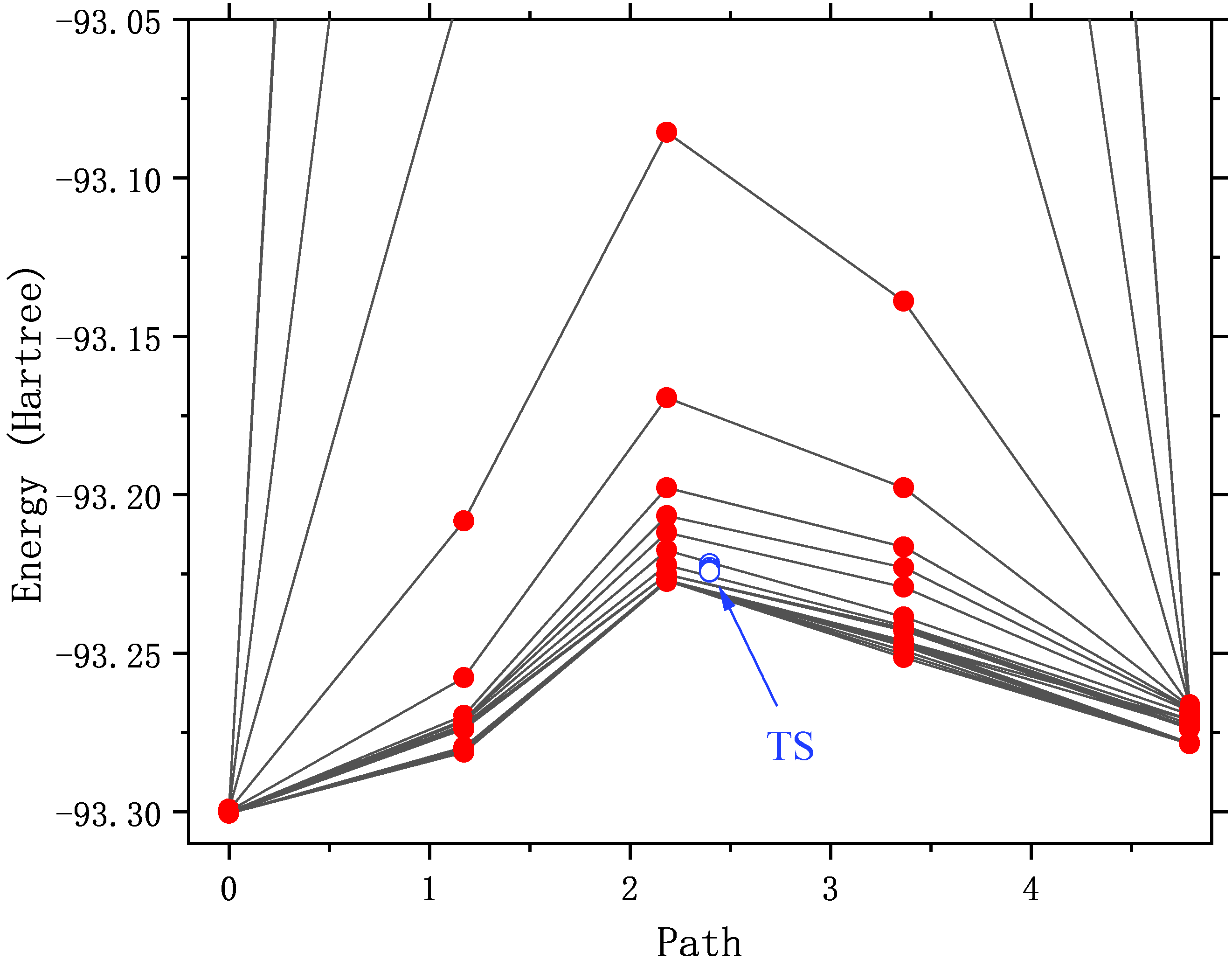
After 31 steps of structural optimization, the CI-NEB method found the lowest energy path:
Testing convergence of NEB climbing image in cycle   31
    Energy  7.1900E-07 Target: 4.0000E-05 converged?  yes
  Max step  1.1193E-03 Target: 5.3333E-03 converged?  yes component     8
  RMS step  6.5514E-04 Target: 3.5556E-03 converged?  yes
  Max grad  7.4900E-05 Target: 1.3333E-03 converged?  yes component     5
  RMS grad  3.6435E-05 Target: 8.8889E-04 converged?  yes
Convergence reached
Scroll forward to see the energy summary report of each image point (including reactants, products, and transition states):
NEB Report
             Energy       F_tang    F_perp     Dist     Angle 1-3 Ang 1-2 Sum
Img    1    -93.3003651   0.00000   0.00000   1.17248    0.00    0.00   63.25   frozen
Img    2    -93.2804319   0.00160   0.00059   1.01235   63.25   86.25   94.29   frozen
Img    3    -93.2270244  -0.00167   0.00049   1.17963   31.04   77.08   80.27   frozen
Img    4    -93.2512597  -0.00248   0.00075   1.42718   49.23    0.00   49.23   frozen
Img    5    -93.2785849   0.00000   0.00000   0.00000    0.00    0.00    0.00   frozen
Cimg   3    -93.2241949   0.00010   0.00007   0.21264    0.00    0.00    0.00
In the table above, the Energy column gives the energy of each image point in the reaction path, where the last Cimg represents the climbing image point, which is the transition state, And the closest image point to it (in this case, image point 3) is marked. The F_tang and F_perp columns give the forces on each image point in the direction of the parallel and perpendicular paths, which should be close to zero in principle. The Dist, Angle, 1-3 Ang, and 1-2 Sum columns give the characteristics of the path, which are the distance from the current image point to the next image point (you can see that the image point of NEB is no longer equally spaced after optimization), The angle of the current image point to the previous image point, the angle of the next image point to the previous image point, and the sum of the angles of the current image point and the next image point. By adding up the data in the Dist column as the horizontal axis and the energy as the vertical axis, you can plot the energy plot of the NEB reaction coordinates (these data can be found in a separate file nebinfo).
The total energy of the transition state given in this line is -93.2241949 Hartree (the final converged energy printed by DL-FIND is also this energy), which is very close to the total energy of the transition state of -93.22419648 Hartree optimized by the previous Dimer method.
The Cartesian coordinates of the transition state can be found before the energy data (atomic units) and are also printed at the end of the text file neb_0006.xyz saved by CI-NEB (since the transition state is the sixth image point in this case) in angstroms. The Cartesian coordinates of the remaining 5 image points are saved in the nebpath.xyz of a text file (unit: angstroms). If necessary, the transition state structure can also be optimized more rigorously using the method described above, which is more efficient than using the strict convergence criterion directly in the CI-NEB calculation.
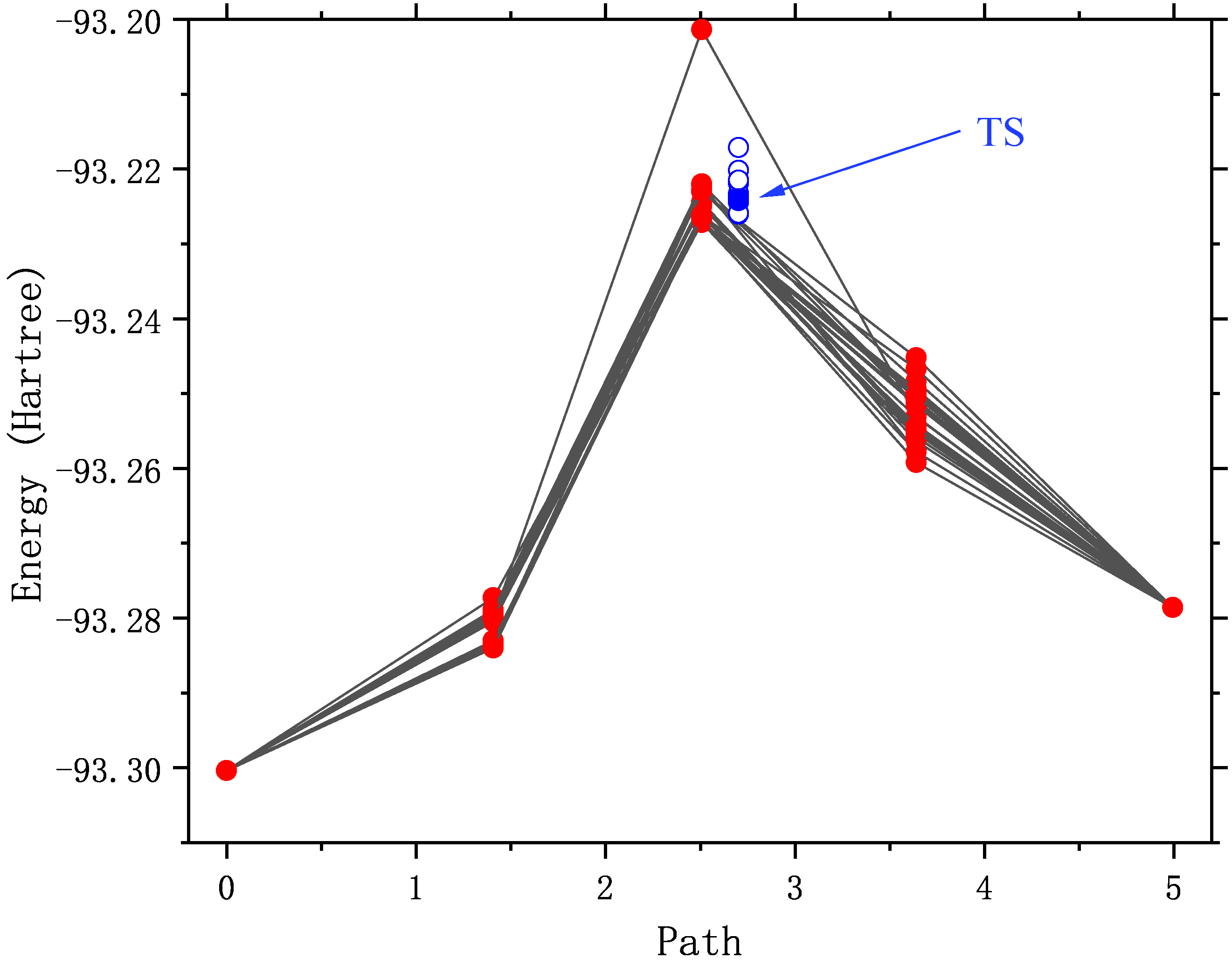
The energy of the optimized image point at each step is extracted, and the NEB trajectory diagram is drawn as follows. As a demonstration, the horizontal coordinates are taken from the last step, but there are actually some variations in the horizontal coordinates for each step.
It can be seen that with the optimization, the energy of the path gradually decreases until it converges. As you may have noticed, the energy of pixels 2 to 4 is very high (out of the display range) in the first few rounds of structural optimization. Illustrates that the initial structure of these points is not quite reasonable. For example, in the initial structure of the No. 3 image spot, the C-N bond is only 0.5 angstrom long! An unreasonable structure will not only hinder the structural convergence, but also destroy the SCF convergence. Or converge to an excited state that we don’t want.
CI-NEB calculations often do not converge. There are the following ways to deal with it:
Extract the structure of the image point with the highest energy or the structure of the climbing image point, and use the transition state optimization method described above to calculate it instead.
Extract the structures of the two image points with the highest energy (e.g., 3 and 4 in this example) as the initial structure, and redo the CI-NEB optimization, but at this time, the “Nebmode” should be changed to 1 or 2, because they are no longer reactants, products, or intermediates, and there is no point in doing energy minimization.
Take the two endpoint structures of the last step of structure optimization, and some or all of the intermediate image point structures (from the data file nebpath.xyz) as the initial structure, and redo the CI-NEB optimization. The input files are as follows. In this example, the structure of both endpoints is already close to convergence (both F_tang and F_perp are very small), and in order to increase the computation speed, the structure remains frozen (Nebmode’ = 2).
$compass
basis-block
 def2-SVP
end basis
geometry
# geom of image 1 (endpoint 1)
C       0.0094403     -0.0045178      0.0000000
N 0.0051489 -1.1595576 0.0000000
H 0.0054108 1.0740754 0.0000000
end geometry
norotate
$end

$bdfopt
solver
 0
iopt
 3
Trust
 0.02
neb-block
 crude
 nebmode
   2
 nimage
   3
end neb
nframe
  4
geometry2
# geom of image 2
C       0.2822075     -0.0905533      0.0000000
N -0.4636856 -0.9729686 0.0000000
H 0.2014782 0.9735219 0.0000000
# geom of image 3
C       0.5703159     -0.2134900      0.0000000
N -0.5233808 -0.6609221 0.0000000
H -0.0269352 0.7844121 0.0000000
# geom of image 4
C       0.7857794     -0.5068651      0.0000000
N -0.3940425 -0.3160241 0.0000000
H -0.3717369 0.7328892 0.0000000
# geom of image 5 (endpoint 2)
C       0.5798873     -0.9890158      0.0000000
N -0.0251869 0.0162146 0.0000000
H -0.5347005 0.8828012 0.0000000
end geometry2
$end

$xuanyuan
$end

$scf
rks
dft
 b3lyp
$end

$resp
 Geom
$end
A little trick is used here: in the automatically generated intermediate image point coordinates, the z-direction coordinates may be non-zero, and in the case of triatomic molecules, the keyword “Norotate” will conflict with the symmetry program. Therefore, the symmetry had to be turned off with “Nosymm” in front. Now that we have qualitatively correct image point coordinates, we can zero out the small values of these coordinates in the z direction. Then change “Nosymm” to “Norotate” so that you can take advantage of the Cs symmetry to speed up the calculation.
Redraw the NEB trajectory as shown in the figure below. Since the intermediate image point uses a good initial structure, the energy in the first few steps of optimization is reasonable.
Structural optimization of spin hybrid states: ZnS molecules
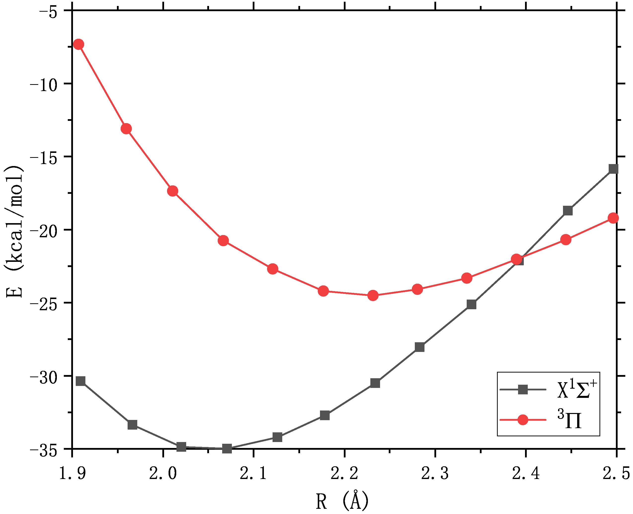
The ground state of the diatomic molecule ZnS is closed-shell :math:’X^1Sigma^+’ with a bond length of 2.05 angstroms, and the first excited state above 11 kcal/mol is math:’^3Pi’, Crossover with the ground state near 2.4 angstrom :cite:’PSS2007’. The :math:’^3Pi_{0+}’ component of the excited state interacts with the ground state, The bond length that may affect the ground state.
If accuracy is not required, the spin-orbit model Hamiltonian proposed by Truhlar et al. can be used to simulate the spin-orbit coupling between two spin states. Consider the effect of :math:’^3Pi_{0+}’ on the ground state. The input files are as follows. Among them, the ground state is completed with RKS, and the lowest triple excited state is completed with UKS. There are a few things to note in the input file:
Note
The option for two-state hybrid computing is “2SoC” (similar to “3SoC”, “4SoC”, etc.). In general, these two spin states need to have different spin multiplicities, unless theoretical calculations prove that there is also a strong SOC interaction between two states with the same spin (e.g., the :math:’^2D_u’ and :math:’^2P_u’ of nitrogen atoms).
The empirical value of the spin-orbit coupling constant set here is 400 :math:’rm cm^{-1}’ which happens to be the default value of the program, so it can be omitted and not written.
Specify the BDF’s built-in optimizer with ‘’solver’’ = 1. You can also use the DL-Find optimizer, but it is generally slower.
The energies and gradients of the two spin states should be saved to the $BDFTASK.egrad.1 and $BDFTASK.egrad.2 files, respectively. As for which state is specified as No. 1 or No. 2, it is entirely up to the user to decide and does not affect the final result.
In the process of BDF structure optimization, the SCF orbital saved in the previous step is used as the initial guess of the current SCF step by default to obtain the fastest SCF convergence. Since the two SCF calculations use different SCF pre-guess orbitals, They need to be backed up as $BDFTASK.scforb.1 and $BDFTASK.scforb.2, respectively. However, when overwriting $BDFTASK.scforb with them for the first time, since the SCF calculation has not yet been performed,
If these two files do not exist, the replication error will occur, and the BDF will stop the calculation when it finds out. In order to block out the error copying message, you need to add
2>/dev/nullto the end of the copy command.The lowest triple excited state can also be calculated by spin flipping using TDDFT, which requires adding some additional keywords to the $tddft’ and $resp’ (see the TDDFT section <TDDFTopt>’). However, TDDFT does not describe the charge transfer state well (this is the case with ZnS) and is not used here.
$COMPASS
Title
 two-state calculation of ZnS
Basis
 lanl2dz
Geometry
 Zn 0.0 0.0 0.0
 S   0.0  0.0  2.05
END geometry
$END

$bdfopt
solver
 1
multistate
 2soc  400
$end

$xuanyuan
$end

%cp $BDF_WORKDIR/$BDFTASK.scforb.1   $BDF_WORKDIR/$BDFTASK.scforb    2>/dev/null || :

$SCF
rks
dft
 pbe0
charge
 0
spinmulti
 1
$END

%cp $BDF_WORKDIR/$BDFTASK.scforb     $BDF_WORKDIR/$BDFTASK.scforb.1

$resp
Geom
$end

%cp $BDF_WORKDIR/$BDFTASK.egrad1     $BDF_WORKDIR/$BDFTASK.egrad.1

%cp $BDF_WORKDIR/$BDFTASK.scforb.2   $BDF_WORKDIR/$BDFTASK.scforb    2>/dev/null || :

$SCF
door
dft
 pbe0
charge
 0
spinmulti
 3
$END

%cp $BDF_WORKDIR/$BDFTASK.scforb     $BDF_WORKDIR/$BDFTASK.scforb.2

$resp
Geom
$end

%cp $BDF_WORKDIR/$BDFTASK.egrad1     $BDF_WORKDIR/$BDFTASK.egrad.2
After the calculation, the optimized spin mixed ground-state bond length is 2.1485 angstroms, which is slightly longer than the bond length of the pure single-weight ground state of 2.1480 angstroms (this value is much larger than the high-precision theoretical value of 2.05 angstroms, because the basis group used in this example is too small). Description :math:’^3Pi_{0+}’ elongates the bond length of the ground state by spin-orbit coupling. The output of the last optimized step shows that :math:’^3Pi_{0+}’ accounts for 0.2% of the spin mixed ground state.
Multi-state calculation
-----------------------

Mixed-spin states by 2 scalar states.

Chi =  400.0 cm^-1 is used to constuct the SO model Hamiltonian.

/tmp/zouwl/BDF-1/test.egrad.1
  E=           -75.49718339
/tmp/zouwl/BDF-1/test.egrad.2
  E=           -75.46038704

Energies and weights of mixed-spin states:
------------------------------------------------------------------
 No.            E(mix)            Weights
------------------------------------------------------------------
  1           -75.49727344        99.8%     0.2%
  2           -75.46029699         0.2%    99.8%
------------------------------------------------------------------
In addition to optimizing the structure of the spin mixed ground state, it is also possible to calculate its vibrational frequency, for which the Hessian of the two spin states needs to be saved to the $BDFTASK.hess.1 and $BDFTASK.hess.2 files, respectively.
If you want to calculate the frequency only on the optimized structure, similar to the input above for the optimized structure, just change “solver” = 1 to “hess” = “only”, and change the backup gradient file “$BDFTASK.egrad1” to the backup Hessian file “$BDFTASK.hess”.
When doing structural optimization + frequency calculation, the input needs to be modified additionally. This is because there is no Hessian file in the optimization process, and there is no gradient file in the frequency calculation process, so you have to use ‘’2>/dev/null || :’’ Mask out messages that are duplicated incorrectly. The input files that work properly are as follows:
$COMPASS
Title
 two-state calculation of ZnS
Basis
 lanl2dz
Geometry
 Zn 0.0 0.0 0.0
 S   0.0  0.0  2.05
END geometry
$END

$bdfopt
solver
 1
multistate
 2soc  400
hess
 final
$end

$xuanyuan
$end

%cp $BDF_WORKDIR/$BDFTASK.scforb.1   $BDF_WORKDIR/$BDFTASK.scforb    2>/dev/null || :
$SCF
rks
dft
 pbe0
charge
 0
spinmulti
 1
$END
%cp $BDF_WORKDIR/$BDFTASK.scforb     $BDF_WORKDIR/$BDFTASK.scforb.1

$resp
Geom
$end

%cp $BDF_WORKDIR/$BDFTASK.egrad1     $BDF_WORKDIR/$BDFTASK.egrad.1   2>/dev/null || :
%cp $BDF_WORKDIR/$BDFTASK.hess $BDF_WORKDIR/$BDFTASK.hess.1 2>/dev/null || :

%cp $BDF_WORKDIR/$BDFTASK.scforb.2   $BDF_WORKDIR/$BDFTASK.scforb    2>/dev/null || :
$SCF
door
dft
 pbe0
charge
 0
spinmulti
 3
$END
%cp $BDF_WORKDIR/$BDFTASK.scforb     $BDF_WORKDIR/$BDFTASK.scforb.2

$resp
Geom
$end

%cp $BDF_WORKDIR/$BDFTASK.egrad1     $BDF_WORKDIR/$BDFTASK.egrad.2   2>/dev/null || :
%cp $BDF_WORKDIR/$BDFTASK.hess $BDF_WORKDIR/$BDFTASK.hess.2 2>/dev/null || :
The main purpose of the polymorphic mixing model is to study polymorphic reactions, optimize the reactants, intermediates, products, transition states of the spin mixed state, and reaction pathways. It provides more information than MECP optimization (e.g., if MECP results in a new transition state, a polymorphic hybrid model can estimate the vibrational frequencies and thermochemical quantities in the vicinity of MECP). When the atoms are not too heavy (before 5d), the polymorphic mixed model has many advantages over the two- or four-component relativistic approach, which strictly considers the rotation-orbit coupling.
Restrictive structure optimization
BDF also supports restricting the value of one or more internal coordinates in structural optimization by adding the constrain keyword to the BDFOPT module. The first line after the constrain keyword is an integer (hereinafter referred to as N), representing the total number of restrictions; Lines 2 to N+1 define each limit. For example, the following input indicates that the distance between the 2nd and 5th atoms is limited for structural optimization (there is not necessarily a chemical bond between these two atoms):
$bdfopt
solver
 1
constrain
 1
 2 5
$end
The following inputs indicate that the distance between the 1st and 2nd atoms is limited to the 2nd atom during the structural optimization, while also limiting the bond angle formed by the 2nd, 5th, and 10th atoms (again, there is no requirement for the 2nd and 5th atoms, or the chemical bonds between the 5th and 10th atoms):
$bdfopt
solver
 1
constrain
 2
 1 2
 2 5 10
$end
The following inputs represent the dihedral angle between the 5th, 10th, 15th, and 20th atoms and the dihedral angle between the 10th, 15th, 20th, and 25th atoms at the time of structural optimization:
$bdfopt
solver
 1
constrain
 2
 5 10 15 20
 10 15 20 25
$end
Note
Even if the numerator coordinates are entered as Cartesian coordinates instead of internal coordinates, the BDF can still be restrictively optimized for the internal coordinates.
When it is necessary to freeze multiple atoms at the same time (for example, to study a surface catalytic reaction using a cluster model, and want to freeze a subset of catalyst atoms), although it is still possible to exhaust all the bond lengths, bond angles, and dihedral angles between these atoms and freeze them one by one, it is troublesome and error-prone when the number of atoms that need to be frozen is large. Therefore, BDF also supports the ability to freeze the Cartesian coordinates of atoms by using the frozen keyword. For example:
$bdfopt
...
frozen
 3 # number of atoms to be frozen
 2 -1
 5 -1
 10 -1
$end
Indicates the freezing of atoms 2, 5, and 10. When using the DL-Find optimizer (i.e., solver=0), -1 can also be replaced with a different number to freeze only one or both of the x, y, and z coordinates of that atom:
  0: free (default)
 -1: frozen
 -2: x frozen only
 -3: and Frozen Only
 -4: With Frozen Only
-23: x and y frozen
-24: X and Z Frozen
-34: Y and Z Frozen
For example
$bdfopt
...
frozen
 4 # number of atoms to be frozen
 3 -1
 4 -1
 5 -1
 6 -4
$end
That is, the Cartesian coordinates of atoms 3~5 and the z coordinates of atom 6 are frozen, but atom 6 can still move freely in the x and y directions.
Note
The program freezes the relative Cartesian coordinates between the atoms specified by the user, and the absolute Cartesian coordinates of the atoms may still change due to the change of the standard orientation of the molecule;
The same calculation can freeze both any number of Cartesian coordinates and any number of inner coordinates.
For the calculation of frozen internal coordinates, the program also supports freezing the inner coordinates to a value that is different from the initial structure. For example, in the following input file, the structure of ethylene oxide is optimized at the M06-2X/6-31+G(d,p)/SMD(water) level, but the length of one of the C-O bonds is limited to 2.0 angstroms:
$compass
Geometry
 C                  0.00000000    0.70678098   -0.40492819
 C                  0.00000000   -0.70678098   -0.40492819
 O                  0.00000000    0.00000000    0.95133348
 H 0.86041653 1.24388179 -0.74567167
 H -0.86041653 1.24388179 -0.74567167
 H 0.86041653 -1.24388179 -0.74567167
 H -0.86041653 -1.24388179 -0.74567167
End Geometry
Basis
 6-31+G(d,p)
MPEC+COSX
$end

$bdfopt
Solver
  1
constraint
 1 # number of constraints
 2 3 = 2.0 # constrain the distance of atom 2 and atom 3 at 2.0 Angstrom
$end

$xuanyuan
$end

$scf
RKS
dft
 M062X
Solmodel
 SMD
solvent
 water
$end

$resp
Geom
$end
In the initial structure, both C-O bonds had a bond length of 1.53 angstroms, but after optimizing convergence, it can be found that the frozen C-O bond has a bond length of exactly 2.00 angstroms (instead of 1.53 angstroms), and the other C-O bond length without freezing is optimized to 1.43 angstroms:
|******************************************************************************|
       Redundant internal coordinates on Angstrom/Degree

  Name         Definition         Value     Constraint
  R1 1 2 1.4907 No
  R2 1 3 1.4332 No
  R3 1 4 1.0917 No
  R4 1 5 1.0917 No
  R5          2   3               2.0000    Yes
  R6 2 6 1.0845 No
  R7 2 7 1.0845 No
  A1 2 1 3 86.29 No
...
In the same calculation, only a part of the coordinates can be assigned, and the rest of the coordinates automatically inherit the values in the initial structure. For example, the following input is valid, indicating that the Cartesian coordinates of atoms 1, 2, and 5 are frozen, and the bond angles of atoms 5-6-8 are frozen, and the dihedral angles of atoms 11-12-13-14 are frozen. For example, if the dihedral angle of atoms 11-12-13-14 in the initial structure is 120 degrees, the dihedral angle of atoms 11-12-13-14 is always 120 degrees in the subsequent structural optimization:
$bdfopt
...
solver
 1
frozen
 3
 1 -1
 2 -1
 5 -1
constrain
 2
 5 6 8 = 60.
 11 12 13 14
$end
Note
The program only supports setting the values of the frozen key length, key angle, and dihedral angle, but does not support setting the Cartesian coordinate value of the frozen atom when freezing the Cartesian coordinates.
When you freeze multiple internal coordinates at the same time and assign values, you need to confirm that the frozen internal coordinates are self-consistent with each other. As an example of internal coordinate inconsistency, consider the following input:
$bdfopt
Solver
  1
constraint
 3
 1 2 = 1.0
 1 3 = 2.0
 2 3 = 4.0
$end
Obviously, these three bond length constraints cannot be met at the same time, because it is not possible to form a triangle from three bonds with bond lengths of 1 angstrom, 2 angstroms, and 4 angstroms. When the program finds that it cannot meet all three conditions at the same time, it prints a warning message:
  q2c_coord_calc: warning: the   1-th constraint cannot be enforced, error =  0.204E+00
Check if the input constraints are mutually contradictory, or numerically ill-posed!
  q2c_coord_calc: warning: the   2-th constraint cannot be enforced, error =  0.200E+00
Check if the input constraints are mutually contradictory, or numerically ill-posed!
  q2c_coord_calc: warning: the   3-th constraint cannot be enforced, error = -0.149E+01
Check if the input constraints are mutually contradictory, or numerically ill-posed!
Finally, because the optimizer could not be solved after restarting the optimizer several times, the program returned an error and exited.
Note
In the above example, it is mathematically impossible to satisfy all the constraints of the inner coordinates at the same time. Sometimes, although it is mathematically possible to satisfy all the constraints at the same time, but the initial structure is too far away from the structure that satisfies the constraints, the program may still not find a structure that satisfies all the constraints at the same time, and print a warning or exit with an error.
Optimization of excited state structure
In addition to optimizing the ground state structure, the BDF program can also optimize the excited state structure, please refer to the relevant section of TDDFT <TDDFTopt> for details, which will not be repeated here.
QM/MM structure optimization
BDF can also use the QM/MM combination method for structural optimization, but unlike pure QM structural optimization, QM/MM structural optimization cannot be completed using the BDFOPT module, but must use the built-in structural optimization function of the pDynamo program. For details, please refer to the QM/MM section <QMMMopt> and will not be repeated here.
Automatically eliminate virtual frequencies
Whether it is to optimize the structure of the minimum point or the transition state, the number of virtual frequencies of the optimized convergence structure is often not consistent with the expectation, which can be divided into three categories: (1) the structure of the optimized minimum point convergence has virtual frequencies; (2) There is more than one imaginary frequency of the structure of the optimized transition state convergence; (3) The structure of the convergence of the optimized transition state has no imaginary frequency. For (1) and (2), BDF can automatically eliminate excess virtual frequencies, for which the keyword ‘’rmimag’’ (or ‘’removeimag’’) needs to be added to the input of the BDFOPT module; This keyword also has a certain effect on the case (3), that is, when there is no virtual frequency in the optimization transition state result, it is possible to find a structure with an imaginary frequency nearby, but the success rate is low. For example, the following input means that the minimum point structure is optimized, and then a frequency calculation is made, and the calculation is terminated if there is no imaginary frequency; If there is a virtual frequency, the molecular structure will be automatically perturbed along the direction of the vibration mode corresponding to the virtual frequency with the largest absolute value, and then continue to optimize, and then do a frequency calculation to verify whether the virtual frequency has been eliminated after optimization and convergence, and so on until all the virtual frequencies are completely eliminated, or the frequency has been calculated 10 times and all the virtual frequencies are still not eliminated:
$bdfopt
solver
1
rmimag
$end
The following input works similarly to the above input, except that a full frequency analysis and thermochemical analysis are performed on the last calculated Hessian:
$bdfopt
solver
1
rmimag
hess
 final
$end
The following input indicates that the transition state structure is optimized (a frequency calculation is done before the optimization begins, to provide the initial Hessian for the structure optimization), followed by a frequency calculation, and the calculation is completed if there is exactly one imaginary frequency. If the number of virtual frequencies is greater than 1, the molecular structure will be automatically perturbed along the direction of the second largest virtual frequency in absolute value, and then continue to optimize, and then do a frequency calculation to verify whether the excess virtual frequencies have been eliminated after optimization convergence, and so on until the number of virtual frequencies is equal to 1. If the number of virtual frequencies is equal to 0, it automatically tries to find a structure with a virtual frequency number equal to 1 nearby, and after optimizing the convergence, the frequency is also recalculated to verify the virtual frequency number, and so on until the virtual frequency number is equal to 1:
$bdfopt
solver
1
rmimag
hess
 init # calculate initial Hessian. If a thermochemistry analysis on the final Hessian is desired, change “init” to “init+final”
iopt
 10 # transition state optimization
$end
The following is a complete example of an optimized equilibrium structure for :math:’ce{ClF3}’ at HFLYP/6-31G(d) level:
$compass
title
 ClF3
basis
 6-31G(d)
geometry
Cl 0.0000000 0.0000000 0.0000000
F -2.966870 0.000000 0.000000
F 1.483435 2.569385 0.000000
F 1.483435 -2.569385 0.000000
end geometry
unit
 bohr
nosymm
$end

$bdfopt
solver
 1
rmimag
hess
 final
$end

$xuanyuan
$end

$scf
rks
dft
 HFLYP
$end

$resp
Geom
$end
The initial structure conforms to the :math:’rm D_{3h}’ symmetry, but because the structure of the expected optimal convergence may have virtual frequencies, it is specified in the ‘’compass’ module with the ‘’’nosymm’’ keyword to be calculated under the :math:’rm C_{1}’ group. The program first converges to the minimum point under the :math:’rm D_{3h}’ point cluster:
|******************************************************************************|
       Redundant internal coordinates on Angstrom/Degree

  Name         Definition         Value     Constraint
  R1 1 2 1.6666 No
  R2 1 3 1.6667 No
  R3 1 4 1.6667 No
  A1 2 1 3 119.99 No
  A2 2 1 4 119.99 No
  A3 3 1 4 120.02 No
  D1 4 1 3 2 179.97 No
  D2 2 1 4 3 179.97 No
  D3 3 1 4 2 -179.97 No

|******************************************************************************|
Then restart the Structure Optimizer:
--- Restarting optimizer ... (10 attempt(s) remaining) ---
Next, the program performs a numerical Hessian calculation and finds that the structure has two imaginary frequencies:
Warning: the number of imaginary frequencies, 2, is different from the desired number, 0!
Therefore, the program perturbates the structure and continues to optimize it in order to eliminate the virtual frequency. Because the angle of an F-Cl-F bond is close to 180°, the redundant internal coordinates need to be reconstructed, resulting in the restart of the structure optimizer. Finally, the convergence yields a T-shaped structure belonging to the :math:’rm C_{2v}’ point group:
|******************************************************************************|
       Redundant internal coordinates on Angstrom/Degree

  Name         Definition         Value     Constraint
  R1 1 2 1.5587 No
  R2 1 3 1.6470 No
  R3 1 4 1.6470 No
  R4 2 4 2.1859 No
  A1 2 1 3 85.95 No
  A2 2 1 4 85.94 No

|******************************************************************************|
Finally, the structure optimizer is restarted for the third time, and the Hessian calculation confirms that the structure has no virtual frequencies, that is, the first two imaginary frequencies have been eliminated. At this point, the entire computation declares convergence:
***************************************  Properties of Normal Modes  ***************************************

Results of vibrations:
Normal frequencies (cm^-1), reduced masses (AMU), force constants (mDyn/A)

                                                  1                                 2                                 3
         Irreps                                  A"                                A'                                A'
    Frequencies                            385.8687                          414.4702                          519.9076
 Reduced masses                             24.3196                           21.5030                           19.4352
Force constants                              2.1335                            2.1764                            3.0952
Note
The program does not guarantee that all excess virtual frequencies will be eliminated in all cases, and even if the program ends normally, the number of virtual frequencies may still be wrong. Therefore, even if the “rmimag” keyword is added, the user still needs to check the number of virtual frequency after the optimization is completed. If the number of virtual frequencies is still not equal to the expected value (i.e., for minimum point optimization, there are still virtual frequencies; Or for transition-state optimization, where there are no virtual frequencies or the number of virtual frequencies is greater than one), you need to manually handle the virtual frequency problem <removeimagfreq>’ subsection :ref:.
If the molecule has point group symmetry, but no ‘’nosymm’’ is specified in the calculation, it may not be possible to completely eliminate all the virtual frequencies, and may even lead to non-convergence of structural optimization. For example, in the above example, if nosymm is not specified, and the calculation is performed under the actual point group of the molecule ( :math:’rm D_{3h}’ ), the optimization will not converge because eliminating the two imaginary frequencies will break the :math:’rm D_{3h}’ symmetry.
The structure obtained by restrictive optimization (regardless of whether it is restricted to Cartesian coordinates or internal coordinates) may (but not necessarily) have imaginary frequencies that cannot be eliminated. In this case, if the number of virtual frequencies is greater than expected, it does not necessarily mean that the current structure is unavailable. By observing the vibration patterns of the virtual frequencies, the user should determine for himself whether the virtual frequencies are caused by the constraints imposed during optimization, and then determine whether these virtual frequencies should be eliminated.
Optimization of conical crossings (CI) and lowest energy crossings (MECP).
To optimize CI and MECP, you need to call the DL-FIND external library :cite:’dlfind2009’, for which you need to add the following keywords to the input of the BDFOPT module
solver
 0
Correspondingly, the ‘’solver 1’’ in each of the above studies means that the BDF’s built-in structural optimization code is used instead of DL-FIND for optimization. In principle, DL-FIND can also be used to optimize minimum points and transition states, but the efficiency is generally not as good as that of BDF’s own code, so DL-FIND should only be called for tasks that are not supported by BDF’s built-in code, such as CI and MECP optimization.
The following is an example input for CI optimization, which calculates the conical intersection of the T1 and T2 states of ethylene:
#----------------------------------------------------------------------
# Gradient projection method for CI between T1 and T2 by TDDFT BHHLYP/6-31G
#

$COMPASS
Title
   C2H4 Molecule test run
Basis
   6-31G
Geometry
 C                  0.00107880   -0.00318153    1.43425054
 C                  0.00066030    0.00195132   -1.43437339
 H 0.05960990 -0.89114967 0.84012371
 H -0.05830329 0.95445870 0.96064844
 H 0.05950228 0.89180839 -0.84311032
 H -0.06267534 -0.95390169 -0.95768311
END geometry
nosymm
$END

$bdfopt
imulti # Optimize CI
 2
maxcycle           # Maximum number of optimization steps
 50
Tolgrad # Convergence criterion for root mean square gradient
 1.d-4
Tolstep # Convergence criterion for root mean square step size
 5.d-3
$end

$xuanyuan
$end

$SCF
RKS
charge
 0
spinmulti
 1
atomorb
DFT
 BHHLYP
$END

$tddft
imethod
 1
ISF
 1
Itda
 1
nroot
 5
idiag
 1
istore
 1
crit_e
 1.d-8
crit_vec
 1.d-6
lefteig
ialda
 4
$end

$resp
Geom
norder
 1
method
 2
iroot
 1
nfiles
 1
$end

$resp
Geom
norder
 1
method
 2
iroot
 2
nfiles
 1
$end

$resp
iprt
 1
QUAD
FNAC
double
norder
 1
method
 2
nfiles
 1
pairs
 1
 1 1 1 1 1 2
$end
Note that this task not only needs to calculate the gradient of T1 and T2 states, but also needs to calculate the non-adiabatic coupling vector between T1 and T2 states (completed by the last RESP module), and the relevant keywords can be found in :d oc:’tddft’, which will not be repeated here. In the input of the BDFOPT module, ‘’imulti 2’’’ stands for Optimized CI. Similar to normal structure optimization tasks, CI optimization outputs the gradient and step length convergence for each step, as well as the energy convergence. For example, the output of the last optimization step of the above study is:
Testing convergence  in cycle    6
    Energy  0.0000E+00 Target: 1.0000E-06 converged?  yes
  Max step  9.0855E-04 Target: 5.0000E-03 converged?  yes component     4
  RMS step  5.6602E-04 Target: 3.3333E-03 converged?  yes
  Max grad  5.5511E-05 Target: 1.0000E-04 converged?  yes component     1
  RMS grad  2.7645E-05 Target: 6.6667E-05 converged?  yes
Converged!
 converged
Similar to the above-mentioned optimization tasks, the convergent CI structure is stored in the .optgeom file with Bohr coordinates. Note that the value of the energy row is always displayed as 0, which does not mean that the energy of the system remains unchanged during CI optimization, but because the convergence of energy will not be used to determine whether the convergence is used in the optimization CI. For the same reason, the keyword “tolene” is not useful for CI optimization (and MECP optimization below).
Here’s an example input file for optimizing MECP:
#----------------------------------------------------------------------
# Gradient projection method for MECP between S0 and T1 by BHHLYP/6-31G
#

$COMPASS
Title
   C2H4 Molecule test run
Basis
   6-31G
Geometry
C            -0.00000141      0.00000353      0.72393424
C             0.00000417     -0.00000109     -0.72393515
H 0.73780975 -0.54421247 1.29907106
H -0.73778145 0.54421417 1.29907329
H 0.73777374 0.54421576 -1.29907129
H -0.73779427 -0.54423609 -1.29906321
END geometry
nosymm
$END

$bdfopt
Multi
 2
maxcycle
 50
tolgrad
 1.d-4
tolstep
 5.d-3
noncouple
$end

$xuanyuan
$end

$SCF
RKS
charge
 0
spinmulti
 1
atomorb
DFT
BHHLYP
$END

$resp
Geom
norder
 1
method
 1
$end

$SCF
DOOR
charge
 0
spinmulti
 3
atomorb
DFT
BHHLYP
$END

$resp
Geom
norder
 1
method
 1
$end
The keywords ‘’imulti 2’’ and ‘’noncouple’’ are specified for MECP optimization. Note that the MECP optimization task only needs to compute the gradient of the two states (in this case, the S0 state and the T1 state), and does not need to calculate the non-adiabatic coupling vector. The output of the MECP optimization task is similar to that of the CI optimization task, and will not be repeated here.
Geometry Optimization FAQs
False frequency issues
Geometry optimization not only requires the structure to converge (i.e., the gradient and step size meet the convergence limit requirements), but also requires that the number of imaginary frequencies of the obtained structure conforms to the expected value, that is, when the minimum value point structure is optimized, the number of imaginary frequencies is 0. When the transition state is optimized, the number of virtual frequencies is 1; If the number of imaginary frequencies is greater than 1, it is a higher-order saddle point. When the actual number of virtual frequencies calculated does not match the expected value, the structure needs to be adjusted and re-optimized. In general, the problem of too many virtual frequencies and a small number of low virtual frequencies can be solved by using the rmimag keyword <rmimag> in small quantities. When the rmimag keyword does not work, you should manually resolve the issue where the number of virtual frequencies does not meet your expectations as follows:
When the actual number of virtual frequencies calculated is less than the expected value, that is, the structure with the number of imaginary frequencies is 0 obtained by optimizing the transition state: at this time, it is generally explained that the qualitative error of the obtained transition state structure is required, and the initial guess structure needs to be re-prepared according to chemical knowledge.
When the actual number of calculated virtual frequencies is greater than the expected value, there are two possible situations: (1) The virtual frequency is caused by the numerical error of the calculation, and it is not real. In this case, it can be solved by increasing the grid point, decreasing the integration truncation threshold, and decreasing various convergence thresholds (such as SCF convergence threshold, structure optimization convergence threshold, etc.). (2) There is indeed a virtual frequency in the system. In this case, the normal mode corresponding to the virtual frequency should be checked from the output file, and the convergent structure should be perturbed along the direction of the normal mode, and then the structure after the disturbance should be used as the initial structure to re-optimize.
Note that it is not possible to determine whether an imaginary frequency is caused by a numerical error based on the frequency calculation results alone, but in general, the smaller the absolute value of the imaginary frequency, the more likely it is to be caused by a numerical error, and vice versa.
Structures obtained by restrictive optimization (regardless of whether they are constrained by Cartesian or internal coordinates) may (but are not necessarily) have virtual frequencies that cannot be eliminated. In this case, if the number of virtual frequencies is greater than expected, it does not necessarily mean that the current structure is unavailable. By observing the vibration patterns of the virtual frequencies, the user should determine for himself whether the virtual frequencies are caused by the constraints imposed during optimization, and then determine whether these virtual frequencies should be eliminated.
Symmetry issues
When the initial structure has the symmetry of the point group above the :math:’rm C_1’ group, the structure optimization may break the point group symmetry, for example, when optimizing the ammonia molecule, the initial structural symmetry of the planar structure is :math:’rm D_{3h}’, the structure optimization may obtain a tapered structure with symmetry of :math:’rm C_{3v}’. By default, BDF enforces the symmetry of the molecular point group, unless there is a first-order Jahn-Teller effect in the system. If the user wants BDF to break the symmetry of the molecule, one of the following methods can be taken:
Still optimized to convergence at high symmetry, then the frequency is calculated. If there is an imaginary frequency, the molecular structure is perturbed according to the method in the previous section to eliminate the imaginary frequency. If the molecule can further reduce the energy by breaking the symmetry, then it should be found that the symmetry of the perturbed molecular structure has been reduced, and the structure should be continued to be optimized with the initial structure.
In the COMPASS module, a subgroup of the molecular point group is specified, and the program will only keep the symmetry of the subgroup unbroken. If the :math:’rm C_1’ group is specified, the program allows the molecular symmetry to be broken in any way, which can maximize the probability of obtaining a low-energy structure, but at the cost of not being able to use the point group symmetry to accelerate the computation, resulting in an increase in the computational cost.
Geometry optimization does not converge
There are a number of factors that contribute to non-convergence of geometric optimizations, including:
Numerical noise in energy and gradient;
The potential energy surface is too flat;
The numerator has more than one stable wave function, and the wave function jumps back and forth between each stable solution during structural optimization, and cannot always converge to the same solution stably;
The molecular structure is not reasonable, such as the wrong coordinate unit (e.g. the unit of the coordinate is Bohr, but the unit specified in the input file is Angstrom, or vice versa), overdrawing or omitting the drawing of atoms, the distance between non-bonding atoms is too close, etc.
For some reactions, there is no transition state (either the activation energy of the forward reaction is 0 or the activation energy of the reverse reaction is 0), and if the user mistakenly believes that there is a transition state and optimizes the transition state, the optimization does not converge or always converges to the wrong structure. Therefore, when the transition state optimization is always non-convergent, the user should consider the possibility that there is no transition state in the current reaction, for example, do a flexible scan to see if the scan curve is monotonic, and if the scan curve is monotonic and smooth throughout the reaction, it can be considered that there is no transition state (provided that the range of bond length/bond angle/dihedral angle of the sweep is large enough and the scan step size is small enough).
Some excited state structure optimizations may be optimized near the tapered intersection. For example, when optimizing the S1 structure, it is sometimes optimized to the vicinity of the S0/S1 cone intersection, because the cone intersection is the only local minimum point nearby, but the potential energy surface is not derivable there, and the gradient of 0 cannot be satisfied, so the structure optimization will oscillate infinitely near the cone intersection. For example, if the fluorescence emission is calculated, and the S0/S1 conical intersection can be directly optimized from the Franck-Condon point on the S1 potential energy surface, it can be considered with some certainty that the S1 state of the system is not fluorescent, because the S1 state is very prone to internal conversion relaxation from the S0/S1 cone intersection to the S0 state. If necessary, the user can instead use :ref:’Optimization algorithm for tapered intersections<CI_MECP>’ to optimize the S0/S1 conical intersection without being affected by the underivability of the potential energy surface at that point.
Some TDDFT structure optimizations may be optimized to regions where the ground-state wave function is unstable on the potential energy surface (e.g., a bond is significantly elongated, resulting in double radical properties), and the program will exit due to the virtual excitation energy of the TDDFT (in rare cases, the regenerating energies) and an error in the RESP module. In this case, the user should try to converge to obtain the stable wave function according to his own calculation purpose, or use TDA instead, or calculate a higher excited state. Note that the results of these methods are not equivalent, and users should make a choice after clarifying their own calculation purpose, and should not blindly believe the results just because one of them solves the problem of virtual activation energy.
In rare cases, optimization fails because the internal coordinates of the program construction contain bond angles close to 180 degrees. As mentioned above, generally speaking, the program will repeatedly try to reconstruct the inner coordinates, and will not return an error exit until it fails to converge after 10 attempts, so the probability of BDF error exit due to internal coordinate problems should be lower than that of many other quantization programs.
If there is no convergence in geometric optimization, or no convergence trend although the maximum number of convergence has not yet been reached, after repeated inspection that the three-dimensional structure of the molecule is correct and reasonable (the so-called reasonable structure includes not only the initial structure provided by the user, such as no missing drawings, multiple drawings, wrong drawing atoms, etc.), but also the optimized structure is reasonable, and there is no congestion and distortion of the structure that does not conform to chemical common sense), and the wave function convergence is normal, you can try the following methods to solve the problem in turn:
Optimize the structure of the last frame of the non-converging task as the initial structure, and start the optimization again. Instead of manually copying the structural coordinates of the last frame into the input file, an easier way is to add the keyword “restart” to the COMPASS module, such as:
$compass
title
 CH3Cl geomopt
basis
 def2-SV(P)
geometry
 C                  2.67184328    0.03549756   -3.40353093
 H 2.05038141 -0.21545378 -2.56943947
 H 2.80438882 1.09651909 -3.44309081
 H 3.62454948 -0.43911916 -3.29403269
 Cl 1.90897396 -0.51627638 -4.89053325
end geometry
restart
$end
Assuming that the file name of the input file is “CH3Cl-opt.inp”, then the program will automatically read the coordinates in “CH3Cl-opt.optgeom” as the initial structure (note that although the program will not use the molecular coordinates in the “geometry” field, the molecular coordinates cannot be deleted). At first glance, this seems to be no different from simply increasing the maximum number of iteration steps of geometric optimization, but in fact the effect of this is often better than simply increasing the maximum number of iteration steps, for example, after optimizing 100 steps and then re-reading the structure and optimizing it for 50 steps, the convergence probability is often higher than that of continuous iteration of 150 steps, because when the structure is re-read and continues to be optimized, the program regenerates the initial Hessian, thus avoiding the accumulated error of the quasi-Newton method of continuous multi-step approximation of Hessian.
Reduce the optimization step size, or trust radius. This can be done by using a trust keyword, such as:
$bdfopt
solver
 1
trust
 0.05
$end
The default confidence radius is 0.3, so the new confidence radius should be less than 0.3. Note that if the program detects that the confidence radius is too small, it will dynamically increase the confidence radius, and to avoid this behavior, you can set the confidence radius to a negative value, such as
$bdfopt
solver
 1
trust
 -0.05
$end
That is, the initial confidence radius is set to 0.05, and it is forbidden to exceed 0.05 during the entire structural optimization process.
For transitional-state optimization, the recalchess keyword can be used to specify that the exact Hessian is recalculated every few steps. as
$bdfopt
solver
 1
iopt
 10
hess
 init
recalchess
 10
$end
Indicates that the exact Hessian is recalculated every 10 steps of the structural optimization, except for the exact Hessian calculation before the structural optimization.
Increase the grid point and reduce the integration truncation threshold and the convergence threshold of SCF, etc., to reduce the numerical error. Note: This method is only useful when the structural optimization is almost convergent but not completely.
Use the DL-Find optimizer instead to optimize the structure in Cartesian coordinates:
$bdfopt
solver
 0
$end
where ‘’solver 0’’ means using the DL-Find optimizer instead of the optimizer that comes with BDF. Since DL-Find optimizes the structure in Cartesian coordinates by default, there is no need to specify the optimization in Cartesian coordinates with additional keywords. This method is suitable for the situation that the program cannot be solved after restarting the optimizer many times because the internal coordinate key angle is close to 180 degrees (at this time, the above solutions should be skipped, and the method should be tried directly, because in this case, the probability of solving the problem by this method is the largest, if the problem cannot be solved, then try the above methods in turn), and it is also suitable for although the program error is not because the bond angle is close to 180 degrees, but the calculation system is not suitable for the description of the internal coordinates, Thus optimizing non-convergence cases (e.g. the system is a large non-covalent cluster).
Before applying the above method, the user should check which of the current non-convergent calculated structure is more reasonable than the initial guess structure provided by the user, and use the more reasonable structure as the first guess structure for subsequent re-optimization. If not only the structure after structural optimization is unreasonable, but also finds that the initial guess structure is also unreasonable, the initial guess structure should be reprepared. This is especially important for transition state optimization, where if the molecular structure is optimized outside the transition state region during the first structural optimization, it will be difficult to re-optimize the structure back to the vicinity of the transition state region no matter what methods are tried later. Therefore, it is not advisable to blindly take the last frame structure of the previous structural optimization (or the initial guess structure of the previous structural optimization) as the initial guess structure of the next optimization without checking whether the structure is reasonable.