Solvation Models
Solvation models are used to calculate interactions between solute and solvent, generally categorized into implicit solvent models (continuous medium models) and explicit solvent models. In BDF, for continuous solvent models, options include IEFPCM, SS(V)PE, CPCM, COSMO, ddCOSMO (domain-decomposition COSMO solvation model), and SMD. For explicit solvent models, the QM/MM method is employed, computed using the pDynamo2.0 program package.
Functionalities supported by BDF solvation models:
PCMs |
Ground state |
Excited state |
|||
|---|---|---|---|---|---|
Single-point |
Gradient |
Hessian |
Single-point |
Gradient |
|
COSMO |
√ |
√ |
√ |
√ |
√ |
CPCM |
√ |
√ |
√ |
√ |
√ |
SS(V)PE |
√ |
√ |
√ |
√ |
√ |
IEFPCM |
√ |
√ |
√ |
√ |
√ |
SMD |
√ |
√ |
√ |
√ |
√ |
Solvent Type Setting
Add the solvent keyword in the SCF module to enable solvation effect calculations. The solvent type (e.g., water) should be specified on the next line.
Example input for formaldehyde in aqueous solution:
$COMPASS
Title
  ch2o Molecule test run
Basis
  6-31g
Geometry
  C    0.00000000    0.00000000   -0.54200000
  O    0.00000000    0.00000000    0.67700000
  H    0.00000000    0.93500000   -1.08200000
  H    0.00000000   -0.93500000   -1.08200000
END geometry
nosymm
unit
 ang
$END

$xuanyuan
$END

$SCF
rks
dft
  b3lyp
solvent   #Solvation calculation switch
  water    #Specify solvent
grid
  medium
$END
Solvent types can be specified using names or aliases from BDF Supported Solvents List. For solvents not listed, input the dielectric constant:
solvent
  user   #User-specified
dielectric
  78.3553   #Input dielectric constant
Solvent Model Setting
Continuous medium models treat the solvent as a polarizable continuous medium with a specific dielectric constant.
BDF currently supports ddCOSMO, COSMO, CPCM, IEFPCM, SS(V)PE, and SMD models. Keywords: ddcosmo, cosmo, cpcm, iefpcm, ssvpe, smd.
Input example:
solvent
  water
solmodel
  IEFPCM   #Solvent model
For COSMO and CPCM, use cosmoFactorK to specify the dielectric screening factor \(f_\epsilon=\frac{\epsilon-1}{\epsilon+k}\). Default: k=0.5 for COSMO, k=0 for CPCM.
cosmoFactorK
  0.5
For SMD, manually specify parameters:
refractiveIndex # Refractive index
  1.43
HBondAcidity # Abraham hydrogen bond acidity
  0.229
HBondBasicity # Abraham hydrogen bond basicity
  0.265
SurfaceTensionAtInterface # Surface tension
  61.24
CarbonAromaticity # Aromaticity
  0.12
ElectronegativeHalogenicity # Halogenicity
  0.24
Note
Using the SMD model disables calculation of non-electrostatic component of solvation free energy, replacing it with SMx series \(\Delta G_{CDS}\).
Cavity Customization
Cavity shape significantly impacts solvation energy. Common cavity types: vdW (van der Waals surface), SES (solvent-excluded surface), SAS (solvent-accessible surface).
BDF defaults to vdW cavity using 1.1× UFF radii. Customize cavity shape for COSMO/CPCM/IEFPCM/SS(V)PE/SMD using:
cavity # Cavity surface generation method
  swig # swig | switching | ses | sphere (default: swig)
uatm # United atom topology method
  false # false | true (default: false)
radiusType
  UFF # UFF | Bondi (default: UFF)
vdWScale
  1.1 # Default: 1.1 (1.1× RadiusType radius)
radii
  1=1.4430 2=1.7500 # Set radius of atom 1 to 1.4430Å, atom 2 to 1.7500Å
  # No spaces around "="; max 128 characters/line; multiple lines allowed
radii
  H=1.4430 O=1.7500 # Set H radius to 1.4430Å, O to 1.7500Å (mix with above)
acidHRadius # Acidic H radius (Å)
  1.2
Cavity Methods:
- switching: Smoothing function for vdW surface grid weights
- swig: Switching/Gaussian (additional Gaussian smoothing)
- sphere: Spherical cavity enclosing molecule
uatm merges H atoms into heavy atoms for cavity formation.
Control grid density with cavityNGrid or cavityPrecision:
cavityNGrid # Max tesserae per atom (adjusted to nearest Lebedev grid)
  302 # Default: 302

# OR

cavityPrecision
  medium # ultraCoarse | coarse | medium | fine | ultraFine (default: medium)
Ground State Solvation Energy Calculation
Typically requires only solvent and solmodel in SCF module.
Example for formaldehyde with SMD model:
$COMPASS
Title
  ch2o Molecule test run
Basis
  6-31g
Geometry
  C    0.00000000    0.00000000   -0.54200000
  O    0.00000000    0.00000000    0.67700000
  H    0.00000000    0.93500000   -1.08200000
  H    0.00000000   -0.93500000   -1.08200000
END geometry
$END

$xuanyuan
$END

$SCF
rks
dft
  gb3lyp
solvent   #Solvation switch
  water    #Solvent
solmodel  #Solvation model
  smd
$END
Note
Use cosmosave to export cavity volume/surface area, tesserae coordinates/charges/areas to .cosmo files. Convert to Gaussian format using $BDFHOME/sbin/conv2gaucosmo.py.
Non-Electrostatic Solvation Energy Calculation
Solvation free energy = Electrostatic (PCM) + Non-electrostatic (\(\Delta G_{cav}\) + \(\Delta G_{dis-rep}\)). Cavitation energy (work to form cavity) uses scaled particle theory (Pierotti-Claverie). Dispersion-repulsion uses pairwise potentials.
Non-electrostatic terms are disabled by default. Enable with:
nonels
  dis rep cav # Dispersion | Repulsion | Cavitation
solventAtoms # Solvent atom counts (molecular formula)
  H2O1 # Default: H2O1 ("1" required to avoid ambiguity)
solventRho # Solvent number density (molecules/ų)
  0.03333
solventRadius # Solvent molecular radius (Å)
  1.385
Note
For cav: Manual solventRho/solventRadius required for non-water solvents.
For dis/rep: Manual solventRho/solventAtoms required for non-water solvents.
Common Solvent Radii:
|----------------------|——-|-----------------|————-|----------|———|---------------------| | Radius (Å) | 1.385 | 2.900 | 2.815 | 1.855 | 2.180 | 2.685 |
Customize radii for dispersion-repulsion/cavitation:
solventAtomicSASRadii # SAS radii for dispersion-repulsion (solvent atoms)
  H=1.20 O=1.50
radiiForCavEnergy # Radii for cavitation energy (solute)
  H=1.4430 O=1.7500 # Same syntax as ``radii``
acidHRadiusForCavEnergy # Acidic H radius for cavitation (Å)
  1.2
Introduction to Nonequilibrium Solvation Theory
Excited-state solvation requires nonequilibrium treatment due to rapid vertical absorption/emission processes. Solvent polarization has: - Fast (electronic) component - Slow (orientational) component
Traditional theories overestimate solvent reorganization energy. BDF implements new theory by Prof. Xiangyuan Li (Int. J. Quantum Chem. 2015, 115(11): 700-721) for state-specific calculations.
Excited State Solvation Effect Calculation
Implicit models handle excited states via: - Linear Response (LR) - State-Specific (SS)
### Vertical Absorption Calculation
Linear Response example:
$COMPASS
Title
  ch2o Molecule test run
Basis
  6-31g
Geometry
  C    0.00000000    0.00000000   -0.54200000
  O    0.00000000    0.00000000    0.67700000
  H    0.00000000    0.93500000   -1.08200000
  H    0.00000000    -0.9350000  -1.08200000
END geometry
nosymm
unit
 ang
$END

$xuanyuan
$END

$SCF
rks
dft
  b3lyp
grid
  medium
solvent
  user      # User-specified
dielectric
  78.3553   # Dielectric constant
opticalDielectric
  1.7778    # Optical dielectric constant
solmodel
  iefpcm
$END

$TDDFT
iroot
  8
solneqlr   # Enable nonequilibrium solvation (LR)
$END
Note
User-specified solvents require opticalDielectric (see BDF Supported Solvents List).
Perturbative State-Specific (ptSS) example:
$COMPASS
Title
  SS-PCM of S-trans-acrolein Molecule
Basis
  cc-PVDZ
Geometry
  C                  0.55794100   -0.45384200   -0.00001300
  H                  0.44564200   -1.53846100   -0.00002900
  C                 -0.66970500    0.34745600   -0.00001300
  H                 -0.50375600    1.44863100   -0.00005100
  C                  1.75266800    0.14414300    0.00001100
  H                  2.68187400   -0.42304000    0.00001600
  H                  1.83151500    1.23273300    0.00002700
  O                 -1.78758800   -0.11830000    0.00001600
END geometry
$END

$xuanyuan
$END

$SCF
rks
dft
  PBE0
solvent
  water
solmodel
  iefpcm
$END

$TDDFT
iroot
  5
istore
  1
$END

$resp
nfiles
  1
method
  2
iroot
  1 2 3
geom
norder
  0
solneqss   # State-specific nonequilibrium
$end
Output snippet:
 -Energy correction based on constrant equilibrium theory with relaxed density
*State   1  ->  0
Corrected vertical absorption energy               =    3.6935 eV
Nonequilibrium solvation free energy               =   -0.0700 eV
Equilibrium solvation free energy                  =   -0.1744 eV
Among them, Corrected vertical absorption energy refers to the excitation energy correction calculated by using the new theory of non-equilibrium solvation developed by Prof. Xiangyuan Li’s group.
In the above example, the vertical absorption energy is \(3.69eV\).
BDF currently also supports the calculation of corrected linear response (cLR), and the following is an input file for calculating the non-equilibrium solvation effect of acrolein molecules in the excited state using cLR:
$COMPASS
Title
  cLR-PCM of S-trans-acrolein Molecule
Basis
  cc-PVDZ
Geometry
  C                  0.55794100   -0.45384200   -0.00001300
  H                  0.44564200   -1.53846100   -0.00002900
  C                 -0.66970500    0.34745600   -0.00001300
  H                 -0.50375600    1.44863100   -0.00005100
  C                  1.75266800    0.14414300    0.00001100
  H                  2.68187400   -0.42304000    0.00001600
  H                  1.83151500    1.23273300    0.00002700
  O                 -1.78758800   -0.11830000    0.00001600
END geometry
$END

$xuanyuan
$END

$SCF
rks
dft
  PBE0
solvent
  water
solmodel
  iefpcm
$END

$TDDFT
iroot
  5
istore
  1
$END

$TDDFT
iroot
  5
istore
  1
solneqlr
$END

$resp
nfiles
  1
method
  2
iroot
  1
geom
norder
  0
solneqlr
solneqss
$end
Locate the output from the first TDDFT section and the cLR output from the resp module:
No.     1    w=      3.7475 eV     -191.566549 a.u.  f=    0.0001   D<Pab>= 0.0000   Ova= 0.4683
    CV(0):    A(  15 )->   A(  16 )  c_i:  0.9871  Per: 97.4%  IPA:     5.808 eV  Oai: 0.4688
    CV(0):    A(  15 )->   A(  17 )  c_i:  0.1496  Per:  2.2%  IPA:     9.144 eV  Oai: 0.4392

...

Excitation energy correction(cLR)                  =   -0.0377 eV
The cLR excitation energy is calculated as: \(3.7475 - 0.0377 = 3.7098\text{eV}\).
### Excited State Geometry Optimization
During geometry optimization, solvent has sufficient time to respond, so equilibrium solvation should be considered.
Use the soleqlr keyword in both tddft and resp modules to enable equilibrium solvation effects. Other input/output details are similar to the TDDFT geometry optimization section and won’t be repeated here.
Phenol molecule example with solvation effects:
$COMPASS
Geometry
  C                 -1.15617700   -1.20786100    0.00501300
  C                 -1.85718200    0.00000000    0.01667700
  C                 -1.15617700    1.20786100    0.00501300
  C                  0.23962700    1.21165300   -0.01258600
  C                  0.93461900    0.00000000   -0.01633400
  C                  0.23962700   -1.21165300   -0.01258600
  H                 -1.69626800   -2.15127300    0.00745900
  H                 -2.94368500    0.00000000    0.02907200
  H                 -1.69626800    2.15127300    0.00745900
  H                  0.80143900    2.14104700   -0.03186000
  H                  0.80143900   -2.14104700   -0.03186000
  O                  2.32295900    0.00000000   -0.08796400
  H                  2.68364400    0.00000000    0.81225800
End geometry
basis
  6-31G
$END

$bdfopt
solver
  1
$end

$XUANYUAN
$END

$SCF
DFT
  gb3lyp
rks
solModel
  iefpcm
solvent
  water
$END

$TDDFT
iroot
  5
istore
  1
soleqlr
$END

$resp
geom
soleqlr
method
  2
nfiles
  1
iroot
  1
$end
Vertical Emission Calculation
In the equilibrium geometry of the excited state, the equilibrium solvation effect of ptSS or cLR is calculated, and the corresponding solvent slow polarization charge is saved. The keyword ‘’emit’’ was added to the SCF module to calculate the non-equilibrium ground state energy. Taking the acrolein molecule as an example, ptSS is used to calculate the excited state, and the corresponding input file is as follows:
$COMPASS
Geometry
  C       -1.810472    0.158959    0.000002
  H       -1.949516    1.241815    0.000018
  H       -2.698562   -0.472615   -0.000042
  C       -0.549925   -0.413873    0.000029
  H       -0.443723   -1.502963   -0.000000
  C        0.644085    0.314498    0.000060
  H        0.618815    1.429158   -0.000047
  O        1.862127   -0.113145   -0.000086
End geometry
basis
  cc-PVDZ
$END

$XUANYUAN
$END

$SCF
DFT
  PBE0
rks
solModel
  iefpcm
solvent
  water
$END

$TDDFT
iroot
  5
istore
  1
#soleqlr
$END

$resp
nfiles
  1
method
  2
iroot
  1
geom
norder
  0
#soleqlr
soleqss
$end

$SCF
DFT
  PBE0
rks
solModel
  iefpcm
solvent
  water
emit
$END
Care needs to be taken to specify ‘’soleqss’’ to calculate the equilibrium solvation effect. The output in the file is:
-Energy correction based on constrant equilibrium theory
*State   1  ->  0
Corrected vertical emission energy                 =    2.8118 eV
Nonequilibrium solvation free energy               =   -0.0964 eV
Equilibrium solvation free energy                  =   -0.1145 eV
The “Corrected vertical emission energy” represents the emission energy correction using Prof. Li’s theory. In this example, vertical emission energy is \(2.81eV\).
When using the cLR calculation, you need to find the output of the first TDDFT in the file, and the cLR output in the resp module, and add it to the difference between the E_tot two scfs to get the final vertical emission energy.
A combination of explicit and implicit solvents was used to calculate the aroused solvation effect
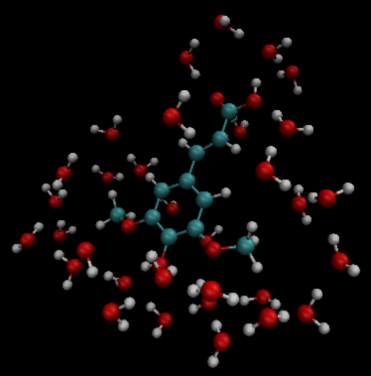
The excited solvation effect can be calculated using a combination of explicit and implicit solvents. In the case of aqueous solutions, it is possible to diffuse to the HOMO and LUMO orbitals of the solute molecules The first hydrate layer, so the water molecules of the first hydrate can be included in the TDDFT calculation area when performing the excited state calculation, while the rest is treated with implicit solvents.
Take sinapic acid, for example. To determine the first hydrate layer of solute molecules, the Amber procedure can be used to perform molecular dynamics simulations by placing the sinapic acid molecules in small water boxes. After the system is equilibrated, the distribution of water molecules around the solute molecules can be analyzed to determine the first hydration layer. Of course, it is also possible to select a multi-frame structure for calculation and then average it.
Hydrate molecule selection can be done using the VMD program. Assuming the input is a pdb file, the first hydrate molecule can be selected in the command line and saved as a pdb file. The command is as follows:
 atomselect top  "same resid as (within 3.5  of not water)"   # Select the first hydrate layer
atomselect0 writepdb sa.pdb                     #The solute molecule and the first hydrate layer are stored in a PDB file
In the example above, all water molecules within 3.5 angstroms of the solute molecule are selected, and as long as one of the three atoms of the water molecule is within the truncated range, the entire molecule is selected. The selection result is shown in the figure:
According to the coordinate information in the sa.pdb file, the TDDFT is calculated, and the input file is as follows:
$COMPASS
Title
 SA Molecule test run
Basis
 6-31g
Geometry
C          14.983  14.539   6.274
C          14.515  14.183   7.629
C          13.251  14.233   8.118
C          12.774  13.868   9.480
C          11.429  14.087   9.838
C          10.961  13.725  11.118
O           9.666  13.973  11.525
C           8.553  14.050  10.621
C          11.836  13.125  12.041
O          11.364  12.722  13.262
C          13.184  12.919  11.700
O          14.021  12.342  12.636
C          15.284  11.744  12.293
C          13.648  13.297  10.427
O          14.270  14.853   5.341
O          16.307  14.468   6.130
H          15.310  13.847   8.286
H          12.474  14.613   7.454
H          10.754  14.550   9.127
H           7.627  14.202  11.188
H           8.673  14.888   9.924
H           8.457  13.118  10.054
H          10.366  12.712  13.206
H          15.725  11.272  13.177
H          15.144  10.973  11.525
H          15.985  12.500  11.922
H          14.687  13.129  10.174
H          16.438  14.756   5.181
O          18.736   9.803  12.472
H          18.779  10.597  11.888
H          19.417  10.074  13.139
O          18.022  14.021   8.274
H          17.547  14.250   7.452
H          18.614  13.310   7.941
O           8.888  16.439   7.042
H           9.682  16.973   6.797
H           8.217  17.162   7.048
O           4.019  14.176  11.140
H           4.032  13.572  10.360
H           4.752  14.783  10.885
O          16.970   8.986  14.331
H          17.578   9.273  13.606
H          17.497   8.225  14.676
O           8.133  17.541  10.454
H           8.419  17.716  11.386
H           8.936  17.880   9.990
O           8.639  12.198  13.660
H           7.777  11.857  13.323
H           8.413  13.155  13.731
O          13.766  11.972   4.742
H          13.858  12.934   4.618
H          13.712  11.679   3.799
O          10.264  16.103  14.305
H           9.444  15.605  14.054
H          10.527  15.554  15.084
O          13.269  16.802   3.701
H          13.513  16.077   4.325
H          14.141  17.264   3.657
O          13.286  14.138  14.908
H          13.185  14.974  14.393
H          13.003  13.492  14.228
O          16.694  11.449  15.608
H          15.780  11.262  15.969
H          16.838  10.579  15.161
O           7.858  14.828  14.050
H           7.208  15.473  13.691
H           7.322  14.462  14.795
O          15.961  17.544   3.706
H          16.342  16.631   3.627
H          16.502  17.866   4.462
O          10.940  14.245  16.302
H          10.828  13.277  16.477
H          11.870  14.226  15.967
O          12.686  10.250  14.079
H          11.731  10.151  14.318
H          12.629  11.070  13.541
O           9.429  11.239   8.483
H           8.927  10.817   7.750
H           9.237  12.182   8.295
O          17.151  15.141   3.699
H          17.124  14.305   3.168
H          18.133  15.245   3.766
O          17.065  10.633   9.634
H          16.918  10.557   8.674
H          17.024   9.698   9.909
O          17.536  14.457  10.874
H          18.014  13.627  11.089
H          17.683  14.460   9.890
O           5.836  16.609  13.299
H           4.877  16.500  13.549
H           5.760  16.376  12.342
O          19.014  12.008  10.822
H          18.249  11.634  10.308
H          19.749  11.655  10.256
O          15.861  14.137  15.750
H          14.900  13.990  15.574
H          16.185  13.214  15.645
O          11.084   9.639  10.009
H          11.641   9.480   9.213
H          10.452  10.296   9.627
O          14.234  10.787  16.235
H          13.668  10.623  15.444
H          13.663  10.376  16.925
O          14.488   8.506  13.105
H          13.870   9.136  13.550
H          15.301   8.683  13.628
O          14.899  17.658   9.746
H          15.674  18.005   9.236
H          15.210  16.754   9.926
O           8.725  13.791   7.422
H           9.237  13.488   6.631
H           8.845  14.770   7.309
O          10.084  10.156  14.803
H           9.498  10.821  14.366
H          10.215  10.613  15.669
O           5.806  16.161  10.582
H           5.389  16.831   9.993
H           6.747  16.470  10.509
O           6.028  13.931   7.206
H           5.971  14.900   7.257
H           6.999  13.804   7.336
O          17.072  12.787   2.438
H          16.281  12.594   1.885
H          17.062  11.978   3.013
END geometry
nosymm
mpec+cosx
$END

$xuanyuan
$end

$SCF
rks
dft
 b3lyp
solvent
 water
grid
 medium
$END

# input for tddft
$tddft
iroot    # Calculate 1 root for each irrep. By default, 10 roots are calculated
  1      # for each irrep
memjkop  # maxium memeory for Coulomb and Exchange operator. 1024 MW (Mega Words)
  1024
$end
A list of solvent types supported in BDF
Name |
Short Name |
\({\epsilon}\) |
\({\epsilon_{opt}}\) |
|---|---|---|---|
water |
H2O |
78.3553 |
1.7764 |
acetic acid |
ACETACID |
6.2528 |
1.8824 |
acetone |
ACETONE |
20.4930 |
1.8463 |
acetonitrile |
ACETNTRL |
35.6880 |
1.8069 |
acetophenone |
ACETPHEN |
17.4400 |
2.3630 |
aniline |
ANILINE |
6.8882 |
2.5163 |
anisole |
ANISOLE |
4.2247 |
2.3025 |
benzaldehyde |
BENZALDH |
18.2200 |
2.3910 |
benzene |
BENZENE |
2.2706 |
2.2533 |
benzonitrile |
BENZNTRL |
25.5920 |
2.3375 |
benzyl chloride |
BENZYLCL |
6.7175 |
2.3688 |
1-bromo-2-methylpropane |
BRISOBUT |
7.7792 |
2.0587 |
bromobenzene |
BRBENZEN |
5.3954 |
2.4327 |
bromoethane |
BRETHANE |
9.0100 |
2.0275 |
bromoform |
BROMFORM |
4.2488 |
2.5616 |
1-bromooctane |
BROCTANE |
5.0244 |
2.1095 |
1-bromopentane |
BRPENTAN |
6.2690 |
2.0872 |
2-bromopropane |
BRPROPA2 |
9.3610 |
2.0309 |
1-bromopropane |
BRPROPAN |
8.0496 |
2.0572 |
butanal |
BUTANAL |
13.4500 |
1.9163 |
butanoic acid |
BUTACID |
2.9931 |
1.9544 |
1-butanol |
BUTANOL |
17.3320 |
1.9580 |
2-butanol |
BUTANOL2 |
15.9440 |
1.9538 |
butanone |
BUTANONE |
18.2460 |
1.9011 |
butanonitrile |
BUTANTRL |
24.2910 |
1.9160 |
butyl acetate |
BUTILE |
4.9941 |
1.9435 |
butylamine |
NBA |
4.6178 |
1.9687 |
n-butylbenzene |
NBUTBENZ |
2.3600 |
2.2195 |
sec-butylbenzene |
SBUTBENZ |
2.3446 |
2.2186 |
tert-butylbenzene |
TBUTBENZ |
2.3447 |
2.2282 |
carbon disulfide |
CS2 |
2.6105 |
2.6631 |
carbon tetrachloride |
CARBNTET |
2.2280 |
2.1319 |
chlorobenzene |
CLBENZEN |
5.6968 |
2.3229 |
sec-butyl chloride |
SECBUTCL |
8.3930 |
1.9519 |
chloroform |
CHCL3 |
4.7113 |
2.0906 |
1-chlorohexane |
CLHEXANE |
5.9491 |
2.0161 |
1-chloropentane |
CLPENTAN |
6.5022 |
1.9957 |
1-chloropropane |
CLPROPAN |
8.3548 |
1.9263 |
o-chlorotoluene |
OCLTOLUE |
4.6331 |
2.3311 |
m-cresol |
M-CRESOL |
12.4400 |
2.3833 |
o-cresol |
O-CRESOL |
6.7600 |
2.3596 |
cyclohexane |
CYCHEXAN |
2.0165 |
2.0352 |
cyclohexanone |
CYCHEXON |
15.6190 |
2.1045 |
cyclopentane |
CYCPENTN |
1.9608 |
1.9782 |
cyclopentanol |
CYCPNTOL |
16.9890 |
2.1112 |
cyclopentanone |
CYCPNTON |
13.5800 |
2.0638 |
cis-decalin |
DECLNCIS |
2.2139 |
2.1934 |
trans-decalin |
DECLNTRA |
2.1781 |
2.1594 |
decalin (cis/trans mixture) |
DECLNMIX |
2.1960 |
2.1765 |
n-decane |
DECANE |
1.9846 |
1.9887 |
1-decanol |
DECANOL |
7.5305 |
2.0655 |
1,2-dibromoethane |
EDB12 |
4.9313 |
2.3676 |
dibromomethane |
DIBRMETN |
7.2273 |
2.3778 |
dibutyl ether |
BUTYLETH |
3.0473 |
1.9578 |
o-dichlorobenzene |
ODICLBNZ |
9.9949 |
2.4072 |
1,2-dichloroethane |
EDC12 |
10.1250 |
2.0874 |
cis-dichloroethylene |
C12DCE |
9.2000 |
2.0996 |
trans-dichloroethylene |
T12DCE |
2.1400 |
2.0892 |
dichloromethane |
DCM |
8.9300 |
2.0283 |
diethyl ether |
ETHER |
4.2400 |
1.8295 |
diethyl sulfide |
ET2S |
5.7230 |
2.0822 |
diethylamine |
DIETAMIN |
3.5766 |
1.9221 |
diiodomethane |
MI |
5.3200 |
3.0363 |
diisopropyl ether |
DIPE |
3.3800 |
1.8712 |
dimethyl disulfide |
DMDS |
9.6000 |
2.3375 |
dimethyl sulfoxide |
DMSO |
46.8260 |
2.0079 |
n,n-dimethylacetamide |
DMA |
37.7810 |
2.0678 |
cis-1,2-dimethylcyclohexane |
CISDMCHX |
2.0600 |
2.0621 |
n,n-dimethylformamide |
DMF |
37.2190 |
2.0463 |
2,4-dimethylpentane |
DMEPEN24 |
1.8939 |
1.9085 |
2,4-dimethylpyridine |
DMEPYR24 |
9.4176 |
2.2530 |
2,6-dimethylpyridine |
DMEPYR26 |
7.1735 |
2.2359 |
1,4-dioxane |
DIOXANE |
2.2099 |
2.0232 |
diphenyl ether |
PHOPH |
3.7300 |
2.4923 |
dipropylamine |
DPROAMIN |
2.9112 |
1.9740 |
n-dodecane |
DODECAN |
2.0060 |
2.0209 |
1,2-ethanediol |
MEG |
40.2450 |
2.0501 |
ethanethiol |
ETSH |
6.6670 |
2.0478 |
ethanol |
ETHANOL |
24.8520 |
1.8526 |
ethyl acetate |
ETOAC |
5.9867 |
1.8832 |
ethyl formate |
ETOME |
8.3310 |
1.8493 |
ethylbenzene |
EB |
2.4339 |
2.2377 |
ethylphenyl ether |
PHENETOL |
4.1797 |
2.2729 |
fluorobenzene |
C6H5F |
5.4200 |
2.1562 |
1-fluorooctane |
FOCTANE |
3.8900 |
1.9418 |
formamide |
FORMAMID |
108.9400 |
2.0944 |
formic acid |
FORMACID |
51.1000 |
1.8807 |
n-heptane |
HEPTANE |
1.9113 |
1.9260 |
1-heptanol |
HEPTANOL |
11.3210 |
2.0303 |
2-heptanone |
HEPTNON2 |
11.6580 |
1.9847 |
4-heptanone |
HEPTNON4 |
12.2570 |
1.9794 |
n-hexadecane |
HEXADECN |
2.0402 |
2.0578 |
n-hexane |
HEXANE |
1.8819 |
1.8904 |
hexanoic acid |
HEXNACID |
2.6000 |
2.0059 |
1-hexanol |
HEXANOL |
12.5100 |
2.0102 |
2-hexanone |
HEXANON2 |
14.1360 |
1.9620 |
1-hexene |
HEXENE |
2.0717 |
1.9146 |
1-hexyne |
HEXYNE |
2.6150 |
1.9569 |
iodobenzene |
C6H5I |
4.5470 |
2.6244 |
1-iodobutane |
IOBUTANE |
6.1730 |
2.2503 |
iodoethane |
C2H5I |
7.6177 |
2.2901 |
1-iodohexadecane |
IOHEXDEC |
3.5338 |
2.1922 |
iodomethane |
CH3I |
6.8650 |
2.3654 |
1-iodopentane |
IOPENTAN |
5.6973 |
2.2377 |
1-iodopropane |
IOPROPAN |
6.9626 |
2.2674 |
isopropylbenzene |
CUMENE |
2.3712 |
2.2246 |
p-isopropyltoluene |
P-CYMENE |
2.2322 |
2.2228 |
mesitylene |
MESITYLN |
2.2650 |
2.2482 |
methanol |
METHANOL |
32.6130 |
1.7657 |
2-methoxyethanol |
EGME |
17.2000 |
1.9667 |
methyl acetate |
MEACETAT |
6.8615 |
1.8534 |
methyl benzoate |
MEBNZATE |
6.7367 |
2.2995 |
methyl butanoate |
MEBUTATE |
5.5607 |
1.9260 |
methyl formate |
MEFORMAT |
8.8377 |
1.8045 |
4-methyl-2-pentanone |
MIBK |
12.8870 |
1.9494 |
methyl propanoate |
MEPROPYL |
6.0777 |
1.8975 |
2-methyl-1-propanol |
ISOBUTOL |
16.7770 |
1.9474 |
2-methyl-2-propanol |
TERBUTOL |
12.4700 |
1.9260 |
n-methylaniline |
NMEANILN |
5.9600 |
2.4599 |
methylcyclohexane |
MECYCHEX |
2.0240 |
2.0252 |
n-methylformamide (E/Z mixture) |
NMFMIXTR |
181.5600 |
2.0503 |
2-methylpentane |
ISOHEXAN |
1.8900 |
1.8810 |
2-methylpyridine |
MEPYRID2 |
9.9533 |
2.2371 |
3-methylpyridine |
MEPYRID3 |
11.6450 |
2.2620 |
4-methylpyridine |
MEPYRID4 |
11.9570 |
2.2611 |
nitrobenzene |
C6H5NO2 |
34.8090 |
2.4218 |
nitroethane |
C2H5NO2 |
28.2900 |
1.9368 |
nitromethane |
CH3NO2 |
36.5620 |
1.9091 |
1-nitropropane |
NTRPROP1 |
23.7300 |
1.9650 |
2-nitropropane |
NTRPROP2 |
25.6540 |
1.9444 |
o-nitrotoluene |
ONTRTOLU |
25.6690 |
2.3870 |
n-nonane |
NONANE |
1.9605 |
1.9751 |
1-nonanol |
NONANOL |
8.5991 |
2.0543 |
5-nonanone |
NONANONE |
10.6000 |
2.0150 |
n-octane |
OCTANE |
1.9406 |
1.9527 |
1-octanol |
OCTANOL |
9.8629 |
2.0435 |
2-octanone |
OCTANON2 |
9.4678 |
2.0025 |
n-pentadecane |
PENTDECN |
2.0333 |
2.0492 |
pentanal |
PENTANAL |
10.0000 |
1.9444 |
n-pentane |
NPENTANE |
1.8371 |
1.8428 |
pentanoic acid |
PENTACID |
2.6924 |
1.9839 |
1-pentanol |
PENTANOL |
15.1300 |
1.9884 |
2-pentanone |
PENTNON2 |
15.2000 |
1.9307 |
3-pentanone |
PENTNON3 |
16.7800 |
1.9388 |
1-pentene |
PENTENE |
1.9905 |
1.8810 |
E-2-pentene |
E2PENTEN |
2.0510 |
1.9025 |
pentyl acetate |
PENTACET |
4.7297 |
1.9664 |
pentylamine |
PENTAMIN |
4.2010 |
2.0967 |
perfluorobenzene |
PFB |
2.0290 |
1.8981 |
phenylmethanol |
BENZALCL |
12.4570 |
2.3704 |
propanal |
PROPANAL |
18.5000 |
1.8594 |
propanoic acid |
PROPACID |
3.4400 |
1.9235 |
1-propanol |
PROPANOL |
20.5240 |
1.9182 |
2-propanol |
PROPNOL2 |
19.2640 |
1.8978 |
propanonitrile |
PROPNTRL |
29.3240 |
1.8646 |
2-propen-1-ol |
PROPENOL |
19.0110 |
1.9980 |
propyl acetate |
PROPACET |
5.5205 |
1.9160 |
propylamine |
PROPAMIN |
4.9912 |
1.9238 |
pyridine |
PYRIDINE |
12.9780 |
2.2786 |
tetrachloroethene |
C2CL4 |
2.2680 |
2.2659 |
tetrahydrofuran |
THF |
7.4257 |
1.9740 |
tetrahydrothiophene-s,s-dioxide |
SULFOLAN |
43.9620 |
2.2002 |
tetralin |
TETRALIN |
2.7710 |
2.3756 |
thiophene |
THIOPHEN |
2.7270 |
2.3375 |
thiophenol |
PHSH |
4.2728 |
2.5259 |
toluene |
TOLUENE |
2.3741 |
2.2383 |
tributyl phosphate |
TBP |
8.1781 |
2.0232 |
1,1,1-trichloroethane |
TCA111 |
7.0826 |
2.0676 |
1,1,2-trichloroethane |
TCA112 |
7.1937 |
2.1650 |
trichloroethene |
TCE |
3.4220 |
2.1824 |
triethylamine |
ET3N |
2.3832 |
1.9628 |
2,2,2-trifluoroethanol |
TFE222 |
26.7260 |
1.6659 |
1,2,4-trimethylbenzene |
TMBEN124 |
2.3653 |
2.2644 |
2,2,4-trimethylpentane |
ISOCTANE |
1.9358 |
1.9363 |
n-undecane |
UNDECANE |
1.9910 |
2.0730 |
m-xylene |
M-XYLENE |
2.3478 |
2.2416 |
o-xylene |
O-XYLENE |
2.5454 |
2.2665 |
p-xylene |
P-XYLENE |
2.2705 |
2.2374 |
xylene (mixture) |
XYLENEMX |
2.3879 |
2.2485 |
1,1-dichloroethane |
10.1900 |
2.0880 |
|
1-iodopentene |
5.7800 |
2.2350 |
|
1-pentyne |
2.0600 |
1.9182 |
|
2-chlorobutane |
8.3900 |
1.9656 |
|
benzyl alcohol |
11.9200 |
2.3716 |
|
bromooctane |
5.0200 |
2.1083 |
|
butyl ethanoate |
5.0700 |
1.9432 |
|
butyl benzene |
2.3600 |
2.2201 |
|
carbon tet |
2.2300 |
2.1316 |
|
chlorotoluene |
6.8500 |
2.3654 |
|
decalin |
2.1900 |
2.1934 |
|
dimethylacetamide |
DMAC |
37.7800 |
2.0678 |
dimethylformamide |
DMF |
37.2200 |
2.0478 |
dimethylpyridine |
7.1700 |
2.2350 |
|
dodecane |
2.0100 |
2.0221 |
|
E-1,2-dichloroethene |
2.1400 |
2.0880 |
|
ethyl ethanoate |
6.0800 |
1.8824 |
|
ethyl methanoate |
8.3300 |
1.8469 |
|
ethyl eneglycol |
40.2500 |
2.0506 |
|
hexadecyl iodide |
3.5300 |
2.1934 |
|
hexanoic |
2.6000 |
2.0051 |
|
isobutanol |
16.7800 |
1.9460 |
|
isopropyl ether |
3.8800 |
1.8714 |
|
isopropyl toluene |
2.2300 |
2.2231 |
|
methyl ethanoate |
6.8600 |
1.8523 |
|
methyl methanoate |
8.8400 |
1.8036 |
|
methyl phenyl ketone |
17.4400 |
2.3624 |
|
methylformamide |
181.5600 |
2.0506 |
|
hexadecane |
2.0600 |
2.0592 |
|
methylaniline |
5.9600 |
2.4649 |
|
pentane |
1.8400 |
1.8414 |
|
pentadecane |
2.0300 |
2.0478 |
|
pentyl ethanoate |
4.7300 |
1.9656 |
|
phenyl ether |
3.7300 |
2.4932 |
|
propyl ethanoate |
5.5200 |
1.9155 |
|
pyrrolidine |
8.0400 |
2.0822 |
|
sec-butanol |
15.9400 |
1.9544 |
|
t-butanol |
12.4700 |
1.9238 |
|
t-butylbenzene |
2.3400 |
2.2290 |
|
tetrahyrothiophenedioxide |
43.9600 |
2.1993 |
|
tribromomethane |
4.2500 |
2.5632 |
|
trichloromethane |
TCM |
4.7100 |
2.0909 |
Z-1,2-dichloroethene |
9.2000 |
2.0996 |
|
isoquinoline |
11.0000 |
1.0100 |
|
quinoline |
9.1600 |
1.0100 |
|
diethylether |
4.2400 |
1.8295 |
|
dichloroethane |
10.1250 |
2.0874 |
|
carbontetrachloride |
2.2280 |
2.1319 |
|
heptane |
1.9113 |
1.9260 |
|
dimethylsulfoxide |
46.8260 |
2.0079 |
|
argon |
1.4300 |
1.4300 |
|
krypton |
1.5190 |
1.5190 |
|
xenon |
1.7060 |
1.7060 |
|
n-octanol |
9.8629 |
2.0435 |
|
aceticacid |
6.2528 |
1.8824 |
|
a-chlorotoluene |
6.7175 |
2.3688 |
|
benzylalcohol |
12.4570 |
2.3704 |
|
butanoicacid |
2.9931 |
1.9544 |
|
butylethanoate |
4.9941 |
1.9435 |
|
carbondisulfide |
2.6105 |
2.6631 |
|
decalin-mixture |
2.1960 |
2.1106 |
|
dibutylether |
3.0473 |
1.9578 |
|
diethylsulfide |
5.7230 |
2.0822 |
|
diisopropylether |
3.3800 |
1.8712 |
|
dimethyldisulfide |
9.6000 |
2.3375 |
|
diphenylether |
3.7300 |
2.4923 |
|
E-1,2-dichloroethene |
2.1400 |
2.0892 |
|
E-2-pentene |
2.0510 |
1.9025 |
|
ethylethanoate |
5.9867 |
1.8832 |
|
ethylmethanoate |
8.3310 |
1.8493 |
|
ethylphenylether |
4.1797 |
2.2729 |
|
formicacid |
51.1000 |
1.8807 |
|
hexanoicacid |
2.6000 |
2.0059 |
|
methylbenzoate |
6.7367 |
2.2995 |
|
methylbutanoate |
5.5607 |
1.9260 |
|
methylethanoate |
6.8615 |
1.8534 |
|
methylmethanoate |
8.8377 |
1.8045 |
|
methylpropanoate |
6.0777 |
1.8975 |
|
n-methylaniline |
5.9600 |
2.4599 |
|
n-methylformamide-mixture |
181.5600 |
2.0503 |
|
n,n-dimethylacetamide |
37.7810 |
2.0678 |
|
n,n-dimethylformamide |
37.2190 |
2.0463 |
|
pentanoicacid |
2.6924 |
1.9839 |
|
pentylethanoate |
4.7297 |
1.9664 |
|
propanoicacid |
3.4400 |
1.9235 |
|
propylethanoate |
5.5205 |
1.9160 |
|
tetrahydrothiophene-s,s-dioxide |
43.9620 |
2.2002 |
|
tributylphosphate |
8.1781 |
2.0232 |
|
xylene-mixture |
2.3879 |
2.2485 |
|
Z-1,2-dichloroethene |
9.2000 |
2.0996 |